This repository implements naive density map to visualize high-dimension data.
This repository includes:
- Dimension reduction of high-dimension data
- Common kernel functions
- Density map generation by kernel estimation
- Visualization of density map
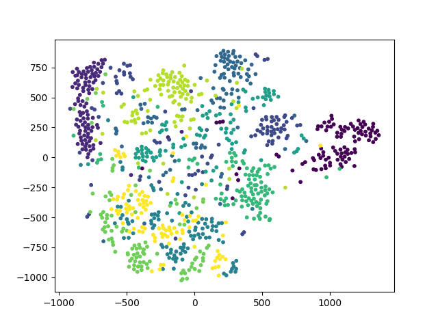
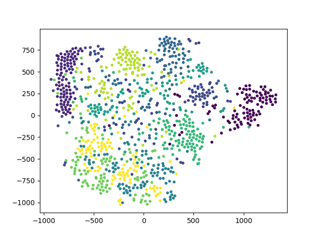
We use common dimension reduction method, i.e., TSNE. However, when dimension grows larger, TSNE is much slower and does not work well. Therefore, we first use PCA to reduce dimension to 100, then use TSNE to reduce dimension to 2.
For efficiency issue, we divide 2-D Euclidean space into grids and count number of points in each grid by class. For
classes, there should be
counting results which are called grid maps. Then we do kernel density estimation on those
grid maps. We notice that KDE can be implemented by convolution operation on the grid maps.
Kernel function is used in kernel density estimation. We implement some common kernel functions:
A 2-D kernel function can be calculated by multiply 1-D kernel functions of x and y dimensions:
In our implementation, we limit the range of Gaussian density estimation by using a Gaussian kernel. All kernel size should be odd number.For classes and grid map of
, we visualize it on a
image where each pixel represent a grid.
Numbers of points in each class may vary greatly. To balance between classes, we first normalize grid maps by class so that maximum value is 1 and minimum value is 0 in each class:
where To represent density of points, we define saturation value of each pixel according to total density of the corresponding grid: where is used to ensure that all saturation value is valid: To show distribution of each class, we use per-pixel color interpolation in HSV color space. For each of the classes, we assign a specific Hue value. Then we calculate hue value of each pixel as weighted sum of all class hue values: We set value of V to 1 for all pixels.Example data of 1000 MNIST images has been put in ./data .
First, create a Python 3.x environment and install following Python packages:
- matplotlib
- numpy
- opencv-python
- scipy
- sklearn
You can install by this shell command:
pip3 install -r requirements.txtTo do dimension reduction, execute:
python dimension_reduction.pyTSNE results are saved into ./tsne folder.
To visualize density map, execute:
python density_map.pyDensity maps are saved into ./result folder.
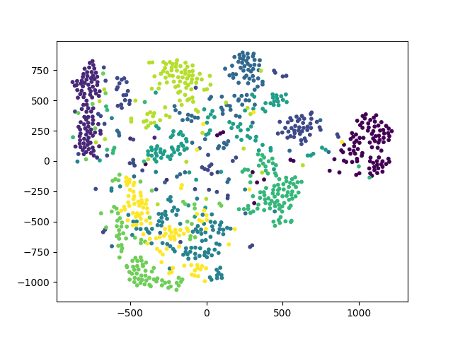
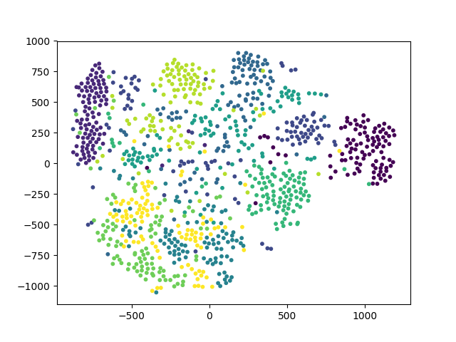
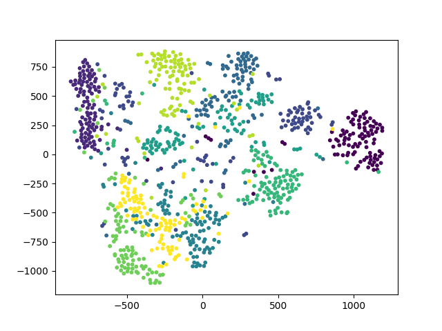
| iter | perplexity=10 | perplexity=30 | perplexity=50 |
|---|---|---|---|
| 250 | 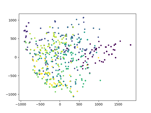 |
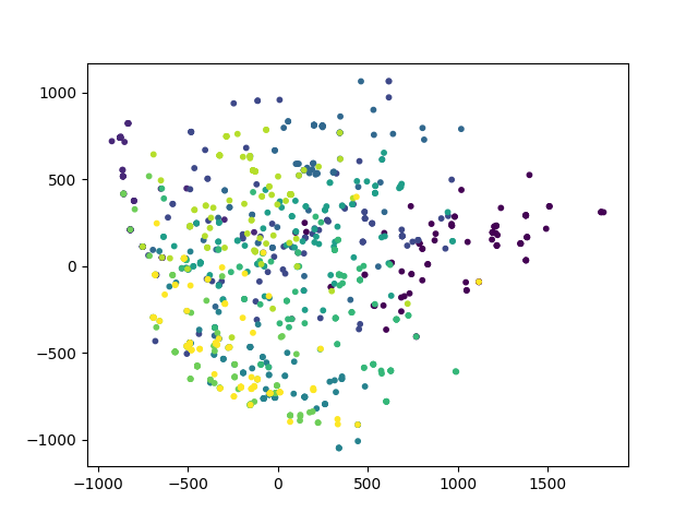 |
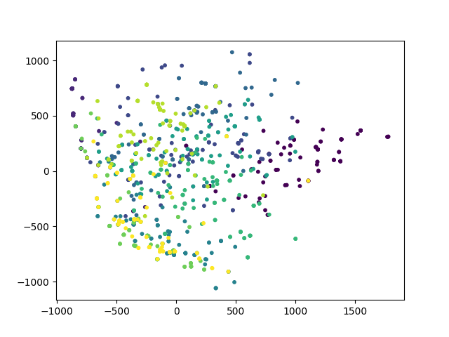 |
| 500 |  |
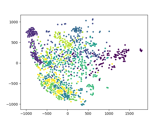 |
 |
| 1000 | 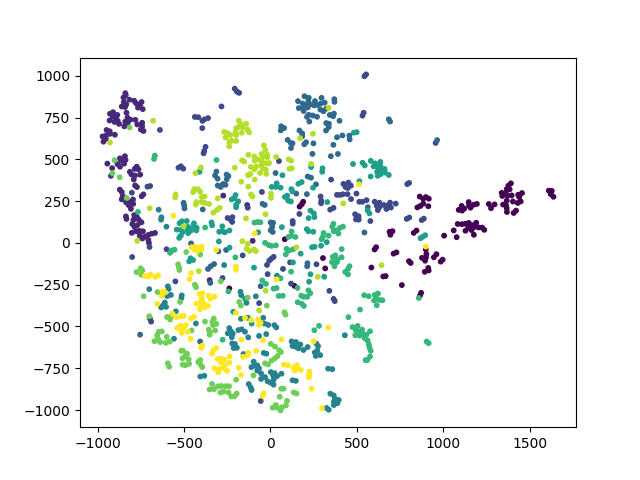 |
 |
 |
| 2000 | 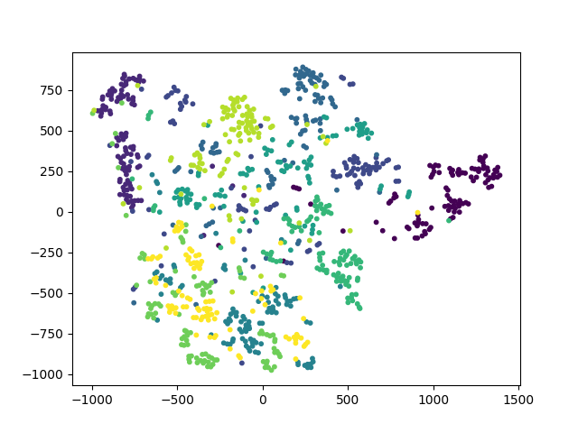 |
 |
 |
| 3500 | 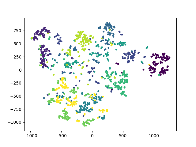 |
 |
 |
| 5000 | 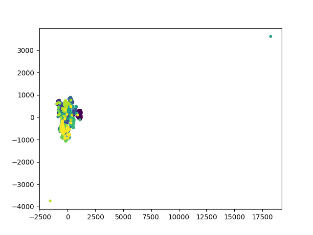 |
 |
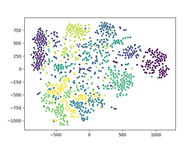 |
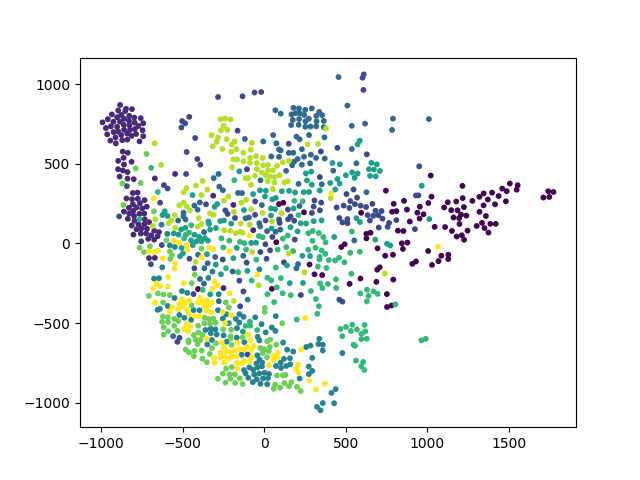
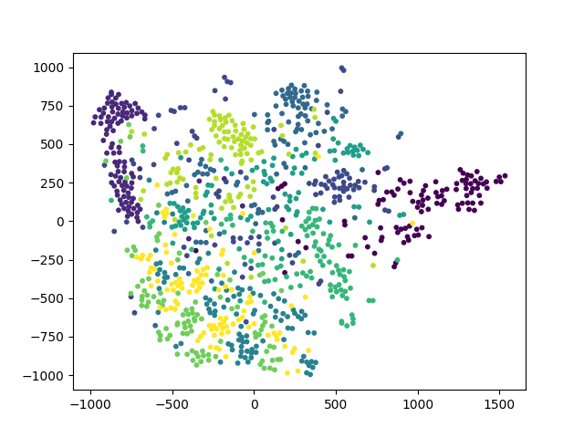
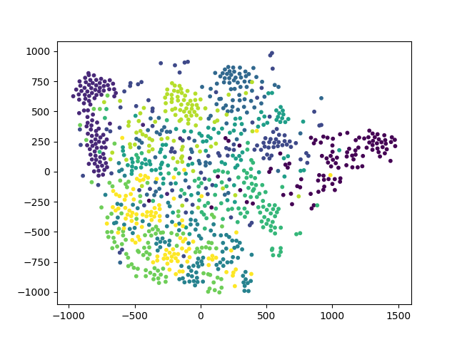
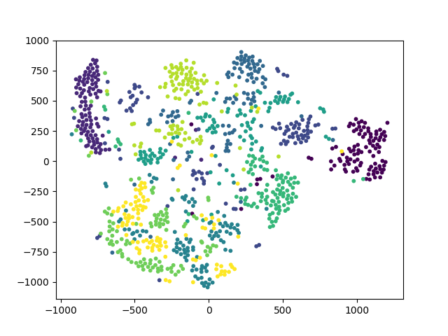
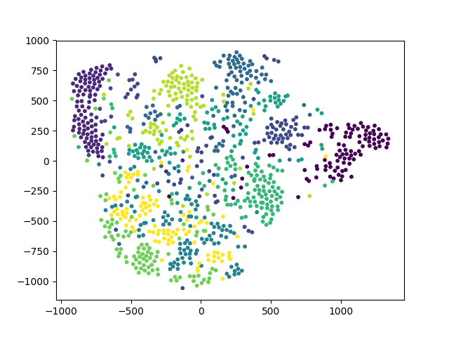
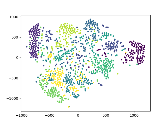
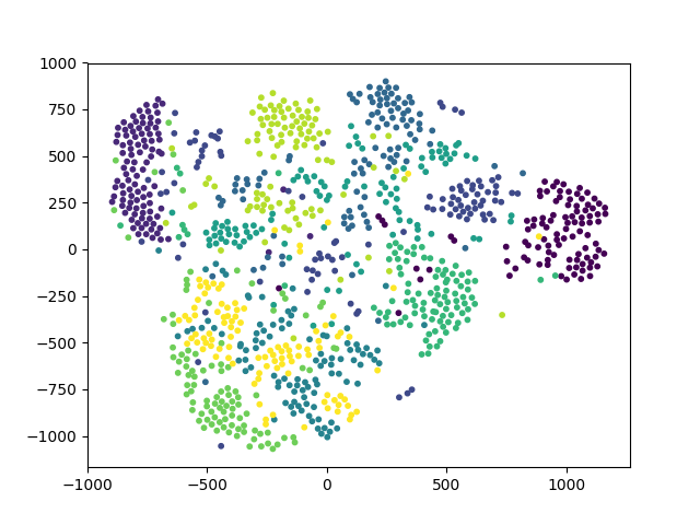
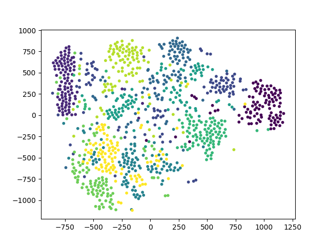
Above results indicate that:
- perplexity=10 is not suitable, perplexity=50 works well.
- number of iterations should be larger than 2000.
We fix perplexity to 30 and 50 respectively.
Perplexity=30:
| Iter | No PCA | PCA (dim=100) | PCA (dim=50) |
|---|---|---|---|
| 2000 |  |
 |
 |
| 3500 |  |
 |
 |
| 5000 |  |
 |
 |
Perplexity=50:
| Iter | No PCA | PCA (dim=100) | PCA (dim=50) |
|---|---|---|---|
| 2000 |  |
 |
 |
| 3500 |  |
 |
 |
| 5000 |  |
 |
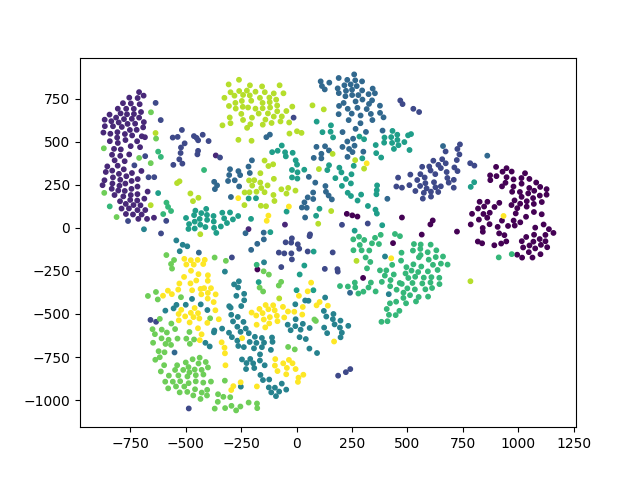 |
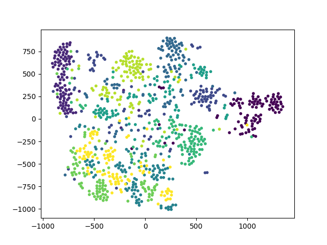
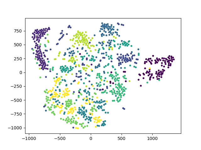
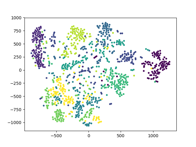
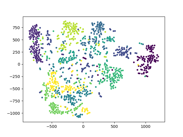
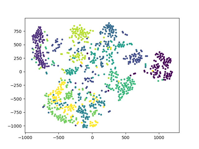
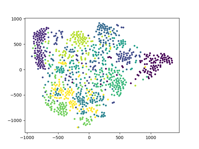
It indicates that PCA preprocessing slightly help separate points of different classes.
We compare efficiency of different methods (in second, perplexity=50):
| iter | TSNE | PCA (dim=100) | PCA (dim=50) | ||||
| Total | PCA | TSNE | Total | PCA | TSNE | Total | |
| 2000 | 10.05 | 0.93 | 8.98 | 9.91 | 0.61 | 8.93 | 9.54 |
| 3500 | 16.00 | 14.88 | 15.81 | 14.77 | 15.38 | ||
| 5000 | 21.76 | 20.65 | 21.58 | 20.57 | 21.18 | ||
It indicates that PCA preprocessing is a litter bit faster than pure TSNE method.
We set and compare visualization results from different kernel functions:
| kernel size | Uniform | Gaussian | Triangular |
|---|---|---|---|
| 7 | .png) |
.png) |
.png) |
| 17 | .png) |
.png) |
.png) |
| 27 | .png) |
.png) |
.png) |
It indicates that uniform kernel produces smoothest density map, while triangular kernel produces sharpest density map.
We use uniform kernel:
| kernel size | |||
|---|---|---|---|
| 7 | .png) |
.png) |
.png) |
| 17 | .png) |
.png) |
.png) |
| 27 | .png) |
.png) |
.png) |
It indicates that using smaller and
(larger grid size) makes density maps smoother. Moreover, with different
and
, suitable kernel size is also changing. Generally, when
and
becomes larger, the suitable kernel size becomes larger and vice versa.
Maaten, Laurens van der, and Geoffrey Hinton. "Visualizing data using t-SNE." Journal of machine learning research 9.Nov (2008): 2579-2605.