-
Data Source Research, Data Cleaning, and Database Storage
- Siyada (Cleaning & Storage)
- Stephan (Data Source Research)
-
Machine Learning
- Stephan
- Siyada
-
Dashboard
- Tesa (Tableau)
- Siyada (HTML/CSS, GitHub Pages)
-
GitHub Repository & Slides
- Tesa
- Siyada
- Stephan
-
Data Cleaning
- Jupyter Notebook 6.4.6
- Python (ETL process)
- Pandas library
- Python (ETL process)
- Quick DBD (Create ERDs)
- PostgreSQL (Join/Merge datasets)
- Jupyter Notebook 6.4.6
-
Database Storage
- pgAdmin 4
- PostgreSQL
- Google Cloud Platform (GCP):
- pgAdmin 4
-
Machine Learning
- Jupyter Notebook or Google Colaboratory (Google Colab Notebook)
- Python
- Prophet
- ARIMA
- LSTM (Keras/TensorFlow)
- Random Forest Regressor
- Python
- Jupyter Notebook or Google Colaboratory (Google Colab Notebook)
-
Dashboard
- Tableau Public 2021.3.3
- Visual Studio Code 1.63.2
- HTML/CSS
- GitHub Pages
-
Slides
- Google Slides
For this project, we intend to develop a robust machine learning model that will deliver a one-year projection for the price of West Texas Intermediate (WTI) Crude Oil, one of the most well-known and widely produced blends of crude in the United States. To do so, we will be examining historical and current data from the Energy Information Agency (EIA), a federal agency that tracks production, sales, and spot & futures prices of WTI Crude. The price projection will be a function of oil production, refinery utilization and capacity, sales, and a variety of other indicators provided by the Energy Information Agency (EIA). We will test four different machine learning methods in order to determine the best fit for this task, shown below: -Random Forest Regression -ARIMA -Prophet LSTM RNN (Recurrent Neural Network)
Many industries, including shipping companies, oil producers, commodities traders, and banks rely heavily upon projections of oil prices to support their decision-making in today’s economy. However, with oil price volatility reaching all-time highs in the past ten years, and with the waning influence of OPEC on the world’s oil production, the task of generating consistent, accurate projections has become increasingly difficult. This has created a considerable opportunity for data scientists and machine learning engineers to apply their skillsets, as well as a demand for complex decision-support systems that firms can employ to navigate the unprecedented dynamics in today’s oil market.
-
Where will the data be sourced from?
-
How will the data be data be transformed and stored?
-
Which machine learning models and libraries should be used?
-
How will the results be visualized?
-
Which model produces the most accurate projections for WTI?
- Gathering data from U.S. Energy Information Administration (EIA)
-
Crude Oil Production dataset
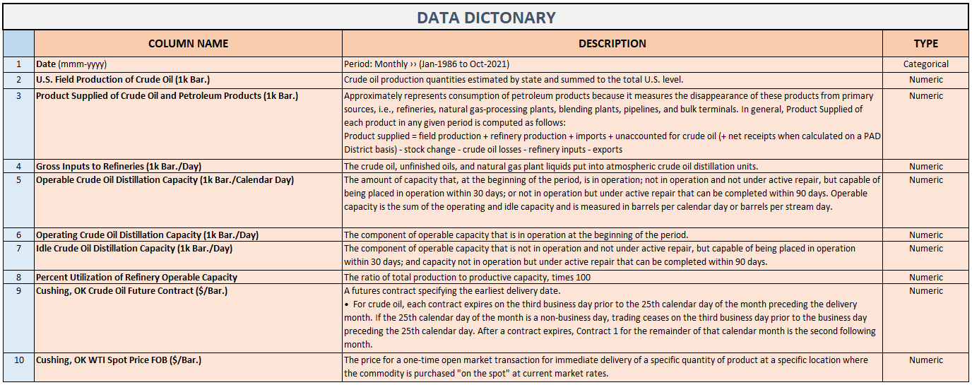
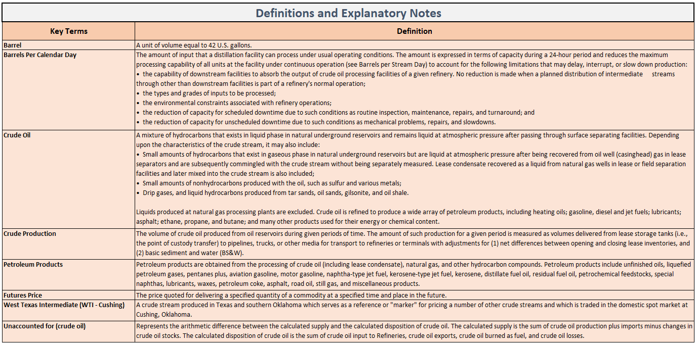
The volume of crude oil produced from oil reservoirs during given periods of time. The amount of such production for a given period is measured as volumes delivered from lease storage tanks (i.e., the point of custody transfer) to pipelines, trucks, or other media for transport to refineries or terminals with adjustments for (1) net
differences between opening and closing lease inventories, and (2) basic sediment and water (BS&W). -
Product Supplied dataset
Approximately represents consumption of petroleum products because it measures the disappearance of these products from primary sources, i.e., refineries, natural gas-processing plants, blending plants, pipelines, and bulk terminals. In general, Product Supplied of each product in any given period is computed as follows: Product supplied = field production + refinery production + imports + unaccounted for crude oil (+ net receipts when calculated on a PAD District basis) - stock change - crude oil losses - refinery inputs - exports
-
Refinery Utilization and Capacity dataset
Ratio of the total amount of crude oil, unfinished oils, and natural gas plant liquids run through crude oil distillation units to the operable capacity of these units.
-
NYMEX Futures Prices dataset
New York Mercantile Exchange, The price quoted for delivering a specified quantity of a commodity at a specified time and place in the future.
-
WTI Crude SPOT Prices Historical dataset
West Texas Intermediate, The price for a one-time open market transaction for immediate delivery of a specific quantity of product at a specific location where the commodity is purchased "on the spot" at current market rates.
-
- There are 5 datasets stored as CSV files
- Crude Oil Production
- Area: U.S.
- Period-Unit: Monthly-Thousand Barrels
- Date: Jan-1920 to Oct-2021
- Product Supplied
- Area: U.S.
- Period-Unit: Monthly-Thousand Barrels
- Date: Jan-1936 to Oct-2021
- Refinery Utilization and Capacity
- Area: U.S.
- Period: Monthly
- Date: Jan-1985 to Oct-2021
- NYMEX Futures Prices
- Area: U.S.
- Period: Daily
- Date: Mar 30, 1983 to Jan 11, 2022
- WTI Crude SPOT Prices Historical
- Area: U.S.
- Period: Daily
- Date: 1/10/2022 to 1/2/1986
- Crude Oil Production
- Create a DataFrame with the columns that we want to keep or Drop unnecessary columns
- Rename the columns by assigning a list of new column names
- Drop the null values using
dropna()method - Convert Data types on "Date" column using
to_datetimemethod - Sort ascending order on "Date" column in the WTI Crude SPOT Prices Historical DataFrame using
sort_valuesmethod - Filter on "Date" column of all DataFrames between (1986-01-01 & 2021-10-31)
- Calculate the average for each month and year in the NYMEX Futures Prices and the WTI Crude SPOT Prices Historical DataFrames
- Round to specific decimals places
- Convert the "Date" column to datetime (in abbreviated Month-Year or mmm-yyyy format) using
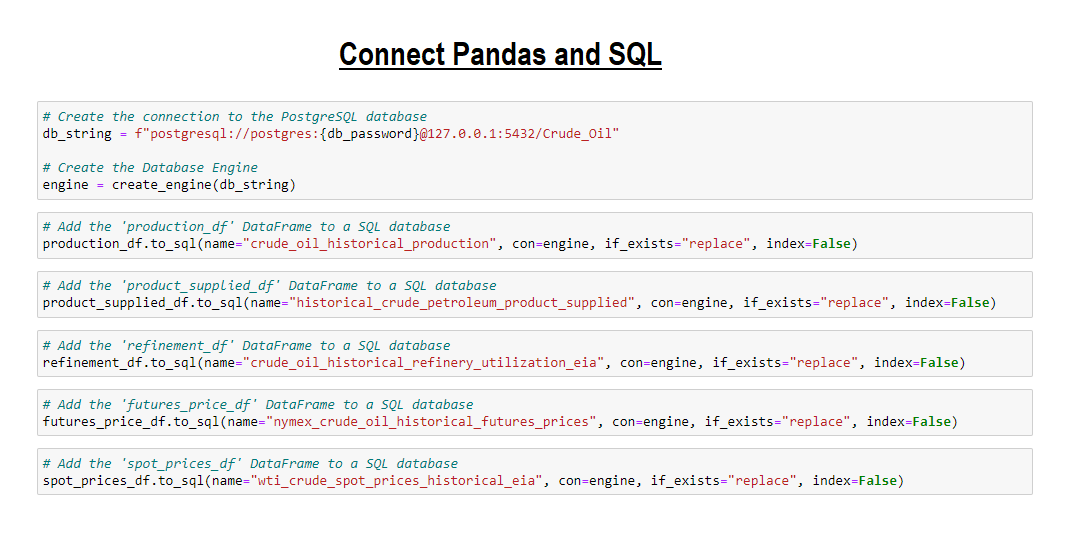
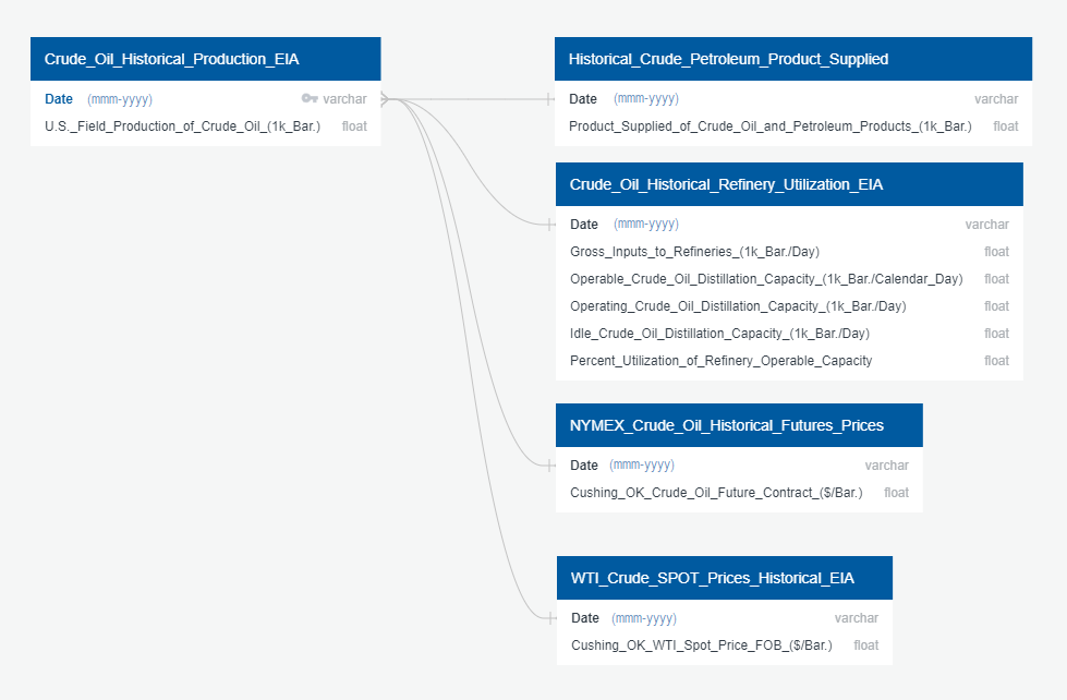
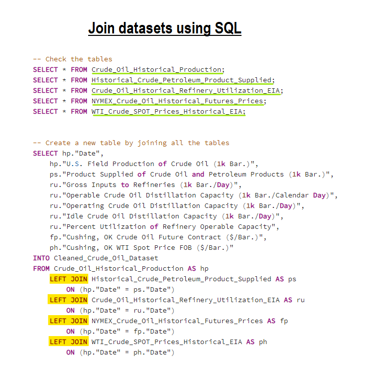
strftime("%b-%Y")method - Join/Merge datasets using PostgreSQL
- Rank the importance of features
- Accuracy
- Random Forest Visualization
- AutoRegressive Integrated Moving Average
- (AR) Regresses target variable on its own prior values.
- lag parameter = p
- (I) Uses differences between observations and their prior values to attempt to make data stationary
- differencing parameter = d
- (MA) Accounts for a moving average of lagged observations
- Moving average window size = q
- Advantages:
- Easy to use when analyzing and creating projections for time-series data
- Drawbacks:
- Potentially ineffective in analyzing data with a non-stationary mean (unit root)
- Extremely sensitive to large shocks
- (AR) Regresses target variable on its own prior values.
- Recurrent Neural Network (RNN)
- Addresses the issue of ‘vanishing gradients’ in neural networks with its gate structure
- Multi-layer networks using certain activation functions experience gradient decay in the loss function, making them harder to train
- Addresses the issue of ‘vanishing gradients’ in neural networks with its gate structure
- Drawbacks:
- Longer model runtime
- Prone to overfitting, especially as depth is added to model
- Forget Gate: Decides which prior inputs are pertinent to the model, and which should be ignored.
- Input Gate: Determines which relevant information can be added from the current step
- Cell State: The path along which information is transported between gates.
- Output Gate: Determines the value of the next hidden state, based on information from input gate and the hidden state.
- Activation Functions: Regulate data in the network, aid in determining if data should be updated or forgotten.
- Developed by Facebook/Meta
- Additive Regression Model
- Includes seasonality component using a Fourier Series: expansion of a periodic function
- Allows the model to more easily account for recurring trends in time series datasets
- Includes seasonality component using a Fourier Series: expansion of a periodic function
- Additive Regression Model
- Drawbacks:
Our Tableau Dashboard has four pages where each dispays detailed visualization of WTI Crude Oil Field Production, Product Supplied of Crude Oil, Petrolium Products, and Future Price analysis.
Here is the sneak peak of the Dashboard:
- In conclusion, our results indicate that Prophet yields the highest accuracy score for forecasting WTI Crude Oil futures, based on the MAPE scores.
- While further improvements can certainly be made to all of these models, Prophet offers an intuitive, user-friendly forecasting platform that boasts impressive accuracy, given its simplicity.
- Random Forest Regressors, particularly when tuned to account for only the most important variables, also serve as a powerful forecasting tool when applied to WTI pricing.
- ARIMA struggles to efficiently cope with the volatility of recent Crude pricing data, as seen in the forecast graph. While the ARIMA calculates a relatively acceptable MAPE, the trend line does not cope well during periods of high price volatility.
- LSTM models have high potential for accurate modeling of financial data, but it appears that the hyperparameters of the model would require extensive tuning in order to be improved.
- Might also benefit from a larger dataset
- Use of weekly or daily data
- Possible increase in model accuracy, at the cost of:
- Increased runtime
- Increased potential for model overfitting
- Possible increase in model accuracy, at the cost of:
- Inclusion of pricing data for historically-correlated asset classes (USD, Gold, etc)
- Caution: in recent years, some of these correlations have shifted
- Inclusion of global oil demand figures, not just product from domestic suppliers
- There are several influences on oil prices
- We could have explored additional data types, such as
- Weather patterns
- Natural disasters
- Political Instability
- Military Conflicts
- Correlated financial instruments
- We could have explored additional data types, such as
- Further exploration of different model types
- VARMA (Vector AutoRegressive Moving Average with differencing)
- Multivariate iteration of ARIMA
- LSTM encoder-decoder Model (interprets data sequence-by-sequence)
- VARMA (Vector AutoRegressive Moving Average with differencing)
- Extrapolation of projections beyond the constraints of the time series
- Considerable scarcity of publicly-available examples/recommendations of how this is accomplished, especially in the case of multivariate, multi-step models
- Deeper understanding of hyperparameter tuning for more complex models
- Would assist in the improvement of model accuracy
- Explore more datasets from various sources and include more categorical data for calculation and visualization.


