For this to work you need to train a model with one of the provided notebooks and move the weights.pt file to /scripts/.
In this project we develop a ROS application capable of taking a single image or a video stream of images with handwritten digits, process it and predict the digit using a neural network. The project is divided in three tasks. Task 1 is responsible for setting the basic structure of the ROS application. In task 2 we develop the synchronization of the topics and the service for the neural network. Finally in task 3, we build and train the model used to predict the digits on the images using pytorch.
ROS is an open-source, meta-operating system for robots. It provides the services from an operating system and also tools and libraries for obtaining, building, writing and running code across multiple computers.
Nodes are one of the core building blocks of ROS. They are executables within a ROS package which can publish or subscribe to topics and can also provide or consume services.
Topics are channels in which messages are published. A node can publish or subscribe to a topic to send or receive messages.
Messages are sent through topics to nodes subscribed to certain topics. Messages can vary from primitive types such as int to custom messages with custom fields and types.
Services are another way that nodes can communicate with each other. Services allow nodes to send a request and receive a response.
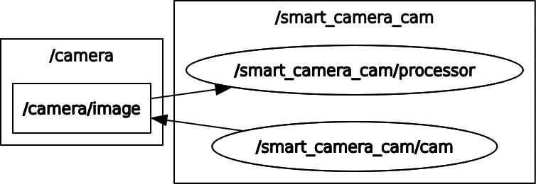
In this task we set up the structure of the project.
- Create a
camand aprocessornodes. - We set up the
camnode to publish 2 topics:/camera/imagewhich publishes an image with a handwritten digit/camera/classwhich publishes the value of the digit with a custom message type
- The
processornode subscribes to the/camera/imageand processes the image. The image is converted to a grayscale image and is cropped. Afterwards the processed image is published to the/processed/imagetopic. - We write a launch file to start both nodes with a single command
At the end of this task, our program structure looks like this:
message_filters is a utility library that collects commonly used message "filtering" algorithms into a common space. The message filters work as follows: a message arrives into the filter and the filter decides whether a message is spit back out at a later point in time or not. An example of a message filter is the Time Synchronizer.
The TimeSynchronizer filter synchronizes incoming channels by the timestamps contained in their headers, and outputs them in the form of a single callback that takes the same number of channels.
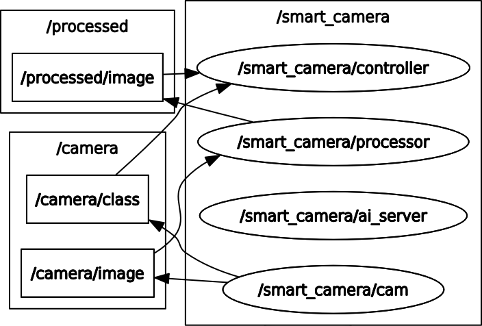
In this task we use the message filter TimeSynchronizer to synchronize our 2 inputs from the controller node. We synchronize the class integer from the /camera/class topic and the processed image from the /processed/image topic.
The integer from the /camera/class topic uses a custom message defined as follow:
# IntWithHeader.msg
Header header
int32 data
The TimeSynchronizer expects a message with a header containing the timestamp at which the message was sent.
When the controller node receives this 2 inputs, this are saved as a python dictionary in an array like this:
{ _class.data: _image }The class being the integer and the image being a numpy array.
For us to be able to predict the handwritten digit in an image, a service is needed. We build a service that takes in an image and outputs an integer, this being the predicted class of the image. Our service file looks like this:
# Ai.srv
sensor_msgs/Image image
---
int32 result
To use the service file we need a server script that handles the logic. For this task the server just takes the image and sends a hardcoded integer. Later in task 3 we will replace this with the actual neural network prediction.
At the end of this task our program structure looks like this:
In this task we create a neural network which takes a handwritten digit image and outputs the digit as an integer. Moreover we modify the ROS application to use the trained neural network.
The goal of a feedforward neural network is to approximate some function $f^$. For example, for a classifier, $y = f^(x)$ maps an input
This network is called feedforward because the information flows through the function being evaluated from
Feedforward neural networks are called networks because they are typically represented by composing together many different functions. For example, we might have 3 functions
Each layer is composed of neurons. Neurons take a set of inputs
An activation function thresholds the output of the neuron within a numerical range. An example of an activation function is the ReLU activation function defined as $ f(x) = max(0, x) $. All negative values are converted to 0 and all positive values are unchanged.
In a fully-connected neural network, all the neurons from a layer are connected with all the neurons in the past and next layer. Neurons within the same layer are not connected with each other. This network architecture is the most used one.
The forward pass of a neural network is computed with matrix multiplications.
Imagine we have a 3 layer fully-connected neural network, the first layer has 128 neurons, the second layer has 64 and the output layer has 10 neurons which corresponds with our 10 digit classes (from 0 to 9).
In the case of our task we have
To get this probabilities in the output layer a function called softmax is a applied to the output values of the last layer. Softmax is defined as $ \sigma(y) = \frac{e^{f_{y_i}}}{\sum_j e_{f_{j_i}}}$, where
A loss function measures how wrong the prediction of our network is. Typically the lower the loss value is, the better is the network prediction. A loss function for classification problems is the cross-entropy loss or log loss. This loss measures the performance of a classification model whose output is a probability value between 0 and 1. Cross-entropy loss increases as the predicted probability diverges from the actual label. So predicting a probability of .012 when the actual observation label is 1 would be bad and result in a high loss value. A perfect model would have a log loss of 0. [2]
The goal of a neural network is to minimize the loss and therefore find the best combination of parameters. One could manually adjust the parameters until a perfect set is found but this would take a lot of time. Instead we can use the partial derivative of the loss function which gives us a gradient. This gradient points in the direction of steepest ascent, if we take the negative of the gradient we can update the parameters by this gradient and through an iterative process arrive at the bottom of the function which corresponds to the best set of parameters. For this task I used the Adam optimizer.
To calculate the partial derivative of very complex functions there is an algorithm called backpropagation. This algorithm uses the chain rule of derivatives to compute gradients at a local level.
Convolutional neural networks (CNN) are a special kind of neural networks which work extremely well with images. In this kind of neural networks the image is not converted to a vector and is left at its original dimensions, in our case
Convolutional neural networks maintain the spatial dimensions, thus they maintain the location of the objects on the images.
For the implementation of the neural network, the framework pytorch was used.
Firstly I imported the MNIST dataset from torchvision.datasets and converted the images to a vector with a Transform. This creates a train and a test split of the dataset. Secondly I created a Dataloader for each split and specified a batch size of 64.
Once the dataset was ready I defined the model. The model is composed of 2 hidden layers and one output layer. The first layer has 128 neurons and the second 64 neurons. Both hidden layers are followed by a ReLU activation function. The output layer has 10 classes corresponding to the digits from 0 to 9, after this layer the values are converted to a probability distribution with softmax.
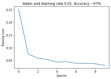
Afterwards I defined the training loop. The model was trained with a cross-entropy loss and the adam optimizer with a learning rate of 0.01 for 10 epochs. After the 10 epochs the model with the lowest loss was saved on a file named weights.pt.
This file was imported in the ROS application for the prediction.
The accuracy of this model is ~97%.
In addition to the fully-connected network, I trained a convolutional neural network to compare the results. The CNN is composed of a single convolutional layer with 32 filters of size
The accuracy of this model is ~98%.
For the application to work with the trained model we have to modify some components. Firstly we need to load an actual MNIST image in the camera node. For this I used cv2.imread and created a helper function to read the image. With the help of the randompackage I generate a random number from 0 to 9, load the corresponding image and publish it on the /camera/image topic. The random generated number is also published on the /camera/class topic.
The processor node listening on the /camera/image topic receives an image and with the help of the method imgmsg_to_cv2(image, 'mono8') from CvBridge, converts the RGB image to a grayscale image. The converted image is then published on the /processed/image topic.
Afterwards we have to modify the ai_server to be able to work with pytorch. After importing all the packages we need to normalize the image, this means to bring all the pixel values to a number between 0 and 1. Also we have to convert the integer values to floats.
Subsequently we need to define a function to generate the model:
def generate_model():
  return nn.Sequential(
    nn.Linear(784, 128),
    nn.ReLU(),
    nn.Linear(128, 64),
    nn.ReLU(),
    nn.Linear(64, 10),
    nn.LogSoftmax(dim=1)
  )
In addition to generating the model we need a function to load and transform the image for pytorch.
def load_image(img):
  loader = transforms.Compose([transforms.ToTensor()])
  return loader(img).float()
After this we create a function to make the actual prediction with the trained model. This function takes an image, loads the trained model and evaluates the image. The output is the integer class value of the image.
The controller node receives the processed image from /processed/image and the ground truth class from /camera/class. With this it sends a request to the ai_servernode which responds with the prediction class. The controller node then outputs both, the ground truth and prediction to the console.
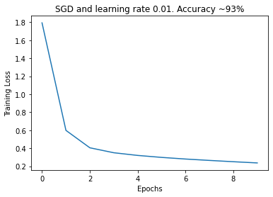
Different optimizers:
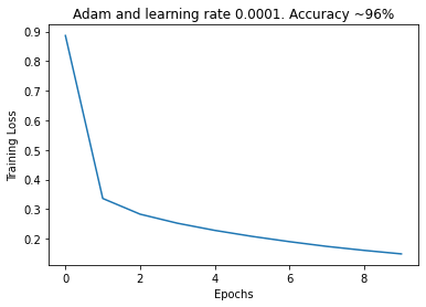
Different optimizers and learning rates:
- Ian Goodfellow, Yoshua Bengio und Aaron Courville. Deep Learning. http://www.deeplearningbook.org. MIT Press, 2016. Visited 05.09.2020
- ML Glossary, Loss functions. [https://ml-cheatsheet.readthedocs.io/en/latest/loss_functions.html#:~:text=Cross%2Dentropy%20loss%2C%20or%20log,diverges%20from%20the%20actual%20label.&text=As%20the%20predicted%20probability%20decreases,the%20log%20loss%20increases%20rapidly](https://ml-cheatsheet.readthedocs.io/en/latest/loss_functions.html#:~:text=Cross-entropy loss%2C or log,diverges from the actual label.&text=As the predicted probability decreases,the log loss increases rapidly.). Visited 05.09.2020.
