Official implementation of paper: Semi-Supervised Learning with Meta-Gradient (AISTATS 2021), by Xin-Yu Zhang, Taihong Xiao, Haolin Jia, Ming-Ming Cheng, and Ming-Hsuan Yang. [paper, poster, video, short slides, full slides]
Under construction.
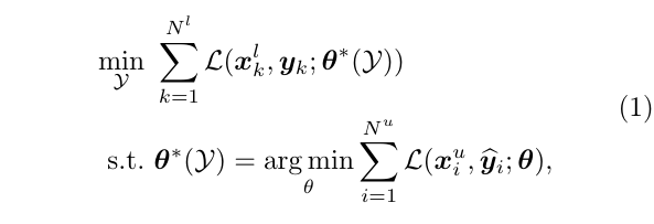
This repository contains the official implementation of the MetaSemi algorithm for Semi-Supervised Learning (SSL). MetaSemi is a consistency-based SSL algorithm in which the consistency loss is guided by the label information of the specific task of interst. However, the consistency loss seems to have no relationship with the label information, so we borrow the idea of meta-learning to establish their relationship by differentiating through the gradient descent step.
we formulate SSL as a bi-level optimization problem, as shown in the following image:
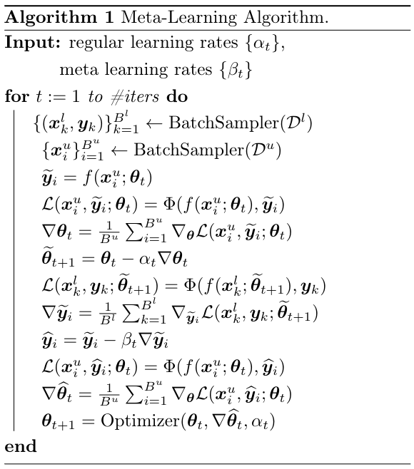
Solving the exact optimization problem is computationally prohibitive, so we adopt an online approximation approach. The MetaSemi algorithm is summarized below:
Apart from meta-learning, we adopt several tricks to alleviate computation overhead and promote performance. Please refer to our paper for these details.
Please make sure the following packages are installed in your environment:
| Package | Version |
|---|---|
| python | >=3.6 |
| pytorch | >=1.2 |
| tensorboardX | >=2.0 |
Also, we provide the Dockerfile containing all necessary dependencies. You can simply run the following commands to enter the docker environment:
cd Docker
sudo docker build .
sudo docker images
sudo docker run <the-image-id> --network=host      # Enter the image id shown in the last command
sudo docker ps
sudo docker exec -it <the-container-id> bash       # Enter the container id shown in the last command
Our performance on SVHN and CIFAR datasets is as follows:
| Dataset | SVHN | CIFAR-10 | CIFAR-100 |
|---|---|---|---|
| Num of Labels | 1000 | 4000 | 10000 |
| Error Rate | 3.15% | 7.78% | 30.74% |
To reproduce these results, run the following commands:
# SVHN
CUDA_VISIBLE_DEVICES='0' python3 train_meta.py --dataset "svhn" --num-label "1000" -a "convlarge" --mix-up --alpha "0.1" --save-path "results/svhn" --seed "7788" --weight-decay "5e-5" --gpu;

# CIFAR-10
CUDA_VISIBLE_DEVICES='0' python3 train_meta.py --dataset "cifar10" --num-label "4000" -a "convlarge" --mix-up --alpha "1.0" --save-path "results/cifar-10" --seed "8469" --weight-decay "1e-4" --gpu;

# CIFAR-100
CUDA_VISIBLE_DEVICES='0' python3 train_meta.py --dataset "cifar100" --num-label "10000" -a "convlarge" --mix-up --alpha "1.0" --save-path "results/cifar-100" --seed "7788" --weight-decay "1e-4" --gpu;
Please omit the --gpu flag and CUDA_VISIBLE_DEVICES='0' prefix if there is no GPU device available.
Our performance on ImageNet dataset is as follows:
| ImageNet | Num of Labels | Top-1 Error | Top-5 Error |
|---|---|---|---|
| ~128k (10%) | 44.87% | 18.88% |
Our ImageNet experiment is based on the NVIDIA-DALI pipeline. Please use the following script to install DALI:
pip3 install --extra-index-url https://developer.download.nvidia.com/compute/redist/cuda/10.0 nvidia-dali==0.13.0
Before running the codes, we need to prepare the ImageNet recorder. You have to download the original ImageNet dataset on your server. Please refer to its official instructions. The downloaded files should be originzed in the following structure:
/your-download-path
├── train
│   ├── n01440764
│   │   ├── n01440764_10470.JPEG
│   │   ├── n01440764_11151.JPEG
│   │   ├── n01440764_12021.JPEG
│   │   ├── ...
│   ├── n01443537
│   │   ├── n01443537_11513.JPEG
│   │   ├── n01443537_12098.JPEG
│   │   ├── n01443537_12507.JPEG
│   │   ├── ...
│   ├── n01484850
│   │   ├── n01484850_10370.JPEG
│   │   ├── n01484850_1054.JPEG
│   │   ├── n01484850_13243.JPEG
│   │   ├── ...
│   ├── ...
├── val
│   ├── n01440764
│   │   ├── ILSVRC2012_val_00000293.JPEG
│   │   ├── ILSVRC2012_val_00002138.JPEG
│   │   ├── ILSVRC2012_val_00003014.JPEG
│   │   ├── ...
│   ├── ...
Then, run the following commands to splits the ImageNet into labeled/unlabeled data:
cd imagenet;
python3 imagenet/split_imagenet.py --data-path "/your-download-path";
After this, there will be four sub-directories under /your-download-path:
/your-download-path
├── train
├── val
├── labeled
├── unlabeled
P.S. Please make sure that your disk have enough space available, since this operation will copy the whole ImageNet (>=150G will be enough). Besides, absolute path is preferred in the above arguments. Running these commands may take a while.
Now, it's time to build the image recorder (See reference). Run the following commands:
# For labeled data
python3 imagenet/im2rec.py /your-download-path/train_label /your-download-path/labeled/ --recursive --list --num-thread 8
python3 imagenet/im2rec.py /your-download-path/train_label /your-download-path/labeled/ --recursive --pass-through --pack-label --num-thread 8

# For unlabeled data
python3 imagenet/im2rec.py /your-download-path/train_unlabel /your-download-path/unlabeled/ --recursive --list --num-thread 8
python3 imagenet/im2rec.py /your-download-path/train_unlabel /your-download-path/unlabeled/ --recursive --pass-through --pack-label --num-thread 8

# For validation data
python3 imagenet/im2rec.py /your-download-path/val /your-download-path/val/ --recursive --list --num-thread 8
python3 imagenet/im2rec.py /your-download-path/val /your-download-path/val/ --recursive --pass-through --pack-label --no-shuffle --num-thread 8
Again, the resulting *.rec files are still copies of ImageNet, so please make sure enough space is available. Finally, under /your-download-path, there should be nine files:
/your-download-path
├── train_label.idx
├── train_label.lst
├── train_label.rec
├── train_unlabel.idx
├── train_unlabel.lst
├── train_unlabel.rec
├── val.idx
├── val.lst
├── val.rec
You only need these nine files to run experiments on ImageNet. Other files are at your disposal.
The following command runs the SSL experiment on ImageNet. We assume eigen GPUs are used in training. The argument --data specifies the directory that contains the above-mentioned nine files.
CUDA_VISIBLE_DEVICES='0,1,2,3,4,5,6,7' python -m torch.distributed.launch --nproc_per_node=8 train_meta_imagenet.py -a "resnet18" --data "/path/to/rec" --save-path "results/imagenet-meta" --batch-size "64" --alpha "1.0";
We also provide script to run the baseline model (labeled-data-only):
CUDA_VISIBLE_DEVICES='0,1,2,3' python3 -m torch.distributed.launch --nproc_per_node=4 train_imagenet.py -a "resnet18" --data "/path/to/rec" --save-path "results/imagenet-baseline" --batch-size "128";
To reproduce Fig. 3 in our paper, run the following commands:
# SVHN
CUDA_VISIBLE_DEVICES="0" python3 plot_features.py --dataset "svhn" --checkpoint-path "results/svhn/model_best.pth" --index-path "results/svhn/label_indices.txt" --save-path "results/svhn/visualization" --num-point '5000';

CUDA_VISIBLE_DEVICES="0" python3 plot_features.py --dataset "cifar10" --checkpoint-path "results/cifar-10/model_best.pth" --index-path "results/cifar-10/label_indices.txt" --save-path "results/cifar-10/visualization" --num-point '5000';
If you find our work intersting or helpful to your research, please consider citing our paper.
@inproceedings{zhang2020semisupervised,
  title = 	 { Semi-Supervised Learning with Meta-Gradient },
  author =       {Zhang, Xin-Yu and Xiao, Taihong and Jia, Haolin and Cheng, Ming-Ming and Yang, Ming-Hsuan},
  booktitle = 	 {Proceedings of The 24th International Conference on Artificial Intelligence and Statistics},
  pages = 	 {73--81},
  year = 	 {2021},
  editor = 	 {Banerjee, Arindam and Fukumizu, Kenji},
  volume = 	 {130},
  series = 	 {Proceedings of Machine Learning Research},
  month = 	 {13--15 Apr},
  publisher =    {PMLR}
}

