Non-Equilibrium Toolbox (NET): For computing confidence bounds on the free-energy estimates computed from non-equilibrium experiments via the Jarzynski equality.
Here is a sample code to compute the confidence bounds on the Jarzynski estimator in 5 easy steps:
# STEP 1: Import toolbox
import sys
sys.path.append('../')

from APIs.NE_ErrorBnds.NE_Error_Bounds import NE_Error_Bounds
from APIs.Models.Random_Data_Generator import Random_Data_Generator

# STEP 2: Set experimental parameters & desired confidence levels
T = 273 + 25 # Experimental temperature in Kelvin
conf_level = 95 # Confidence Level on the Bounds in Percentage

# STEP 3: Initialize the toolbox
RDGObj = Random_Data_Generator(T)
NEBObj = NE_Error_Bounds(T)

# STEP 4: Generate work samples (replace STEP 4 with actual data)
N_samp = 1e3 # No. of work samples
wd_mean = 10 # Measured in KbT
dF_true = 20 # Ground truth Free Energy Change in KbT
wd = RDGObj.get_wd_dist(wd_mean, N_samp) # Generating dissipation work distribution
w = wd + dF_true # Finding the work distribution

# STEP 5: Compute bounds on dF & an estimate of dF
[dF_lower_bound, dF_upper_bound] = NEBObj.get_neq_error_bounds(w, conf_level) # Bounds

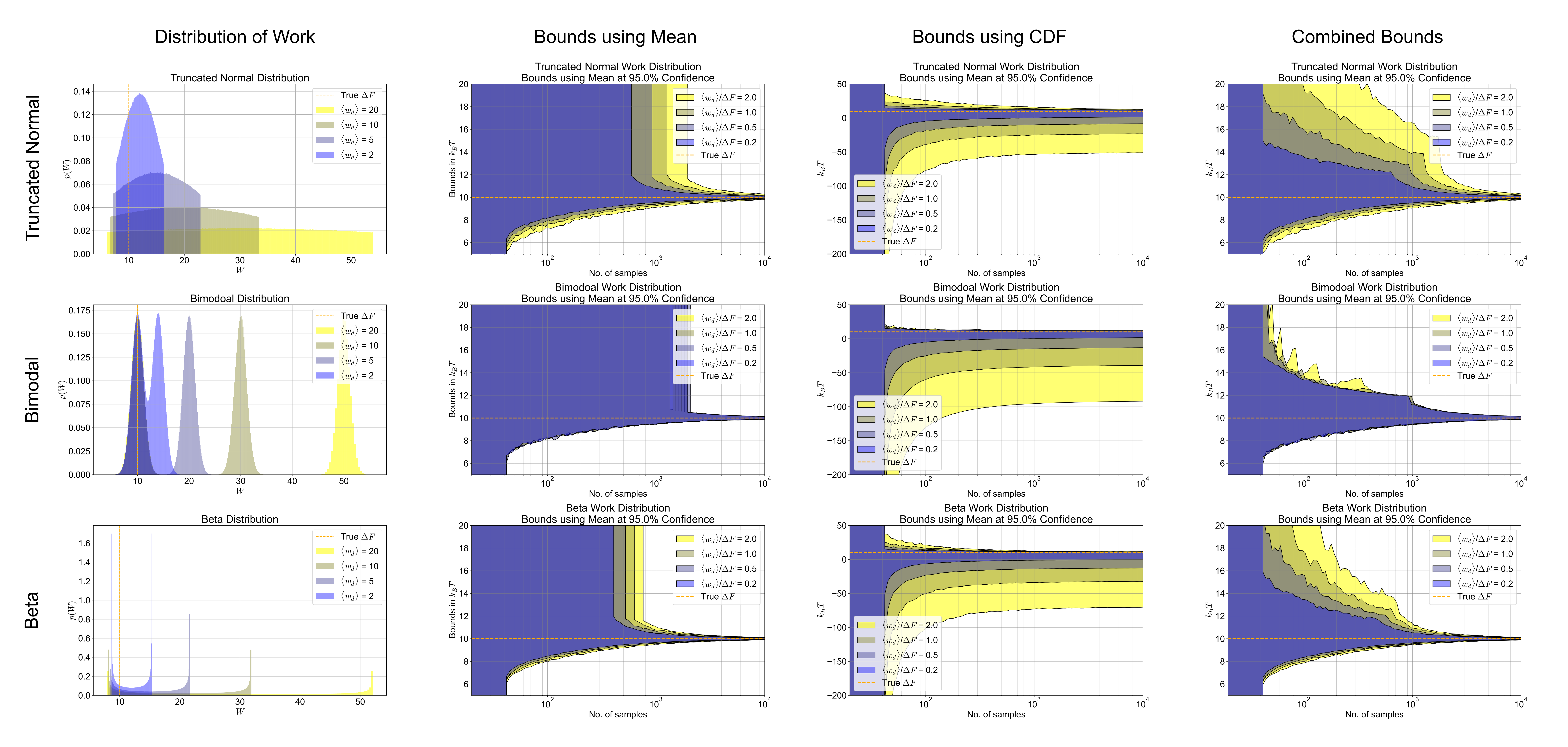
dF_estimate = NEBObj.get_Jarzynski_estimate(w) # dF estimateA summary of the performance and characteristics of the bounds on the synthetic data. (Upper) A detailed view of the performance results. The box plot shows (left) showcases the performance of the Combined Bounds at
The Jarzynski equality links the equilibrium free energy differences between two states of a system to the non-equilibrium work required to move the system between the states.This is given by
The following video shows an illustrative example of the Jarzynski example. In the top left, the schematic of the spring mass system is shown with the blue particle being the externally controlled variable and the green particle being the mass. As the blue particle is stretching according to the top middle plot, the position and the velocity of the mass can be seen in the middle left and bottom left plots. The phase space of the mass can be seen in the center plot. The work done along the trajectory is in the middle bottom plot while the blue particle is stretching. The top right plot is showing work done along multi trajectories and the bottom right plot repeats showing the phase space of hundred of particles. The middle right figure shows the histogram of work done for the whole trajectory, which is approximately Gaussian distributed.
Spring_Mass.mp4
To cite this toolbox, please use:
- Rajaganapathy, Sivaraman, and Murti Salapaka. "Confidence bounds for the Jarzynski estimator." Bulletin of the American Physical Society (2022).

