The Quantum Optomechanics Toolbox

A library of modules for computational quantum optomechanics... and beyond!

The Quantum Optomechanics Toolbox (packaged as qom) is a wrapper-styled, scalable toolbox featuring multiple modules for the calculation of stationary as well as dynamical properties of many-body quantum optomechanical systems. Backed by numerical libraries like NumPy and SciPy, and featuring the highly customizable visualizations offered by Matplotlib and Seaborn APIs, the toolbox aims to serve as an easy-to-use alternative to writing code explicitly and avoiding repetitive exercises for presentable visuals.

Key Features!

Run automatically-managed loops in parallel and pool results.
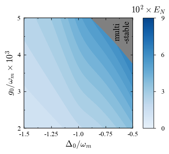
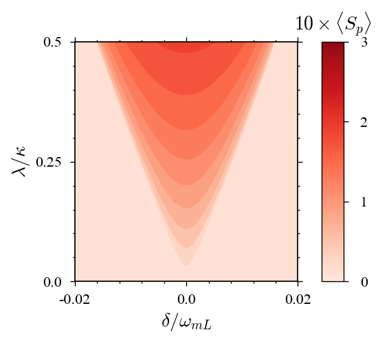
Solve for stability and classical/quantum signatures seamlessly.
Configure plots across plotting libraries with a common syntax.

What's New in v1.0!

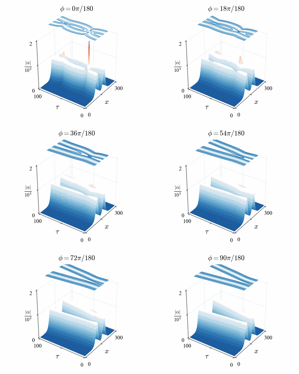
Non-linear Schrodinger equation solver with integration support.
Attractor detection and bifurcation for non-linear dynamical systems.
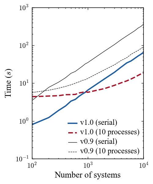
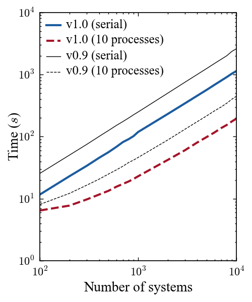
Huge performance boost with NumPy-based vectorization.
Faster Monte-Carlo quantum trajectories solver for low-dimensional Hilbert spaces (deprecated since qom-v1.0.2).

Dynamical Stability	Quantum Correlations

Runtimes for the calculation of dynamical stability of the steady state using the Routh-Hurwitz criteria.	Runtimes for the calculation of average entanglement from the dynamical values of modes and correlations.

Examples

Classical Amplitudes	Quantum Fluctuations

The classical mean values of the optical and mechanical modes are obtained using the rate equations of the modes.	The variances of the quantum fluctuation quadratures are obtained using the rate equation for the correlation matrix.

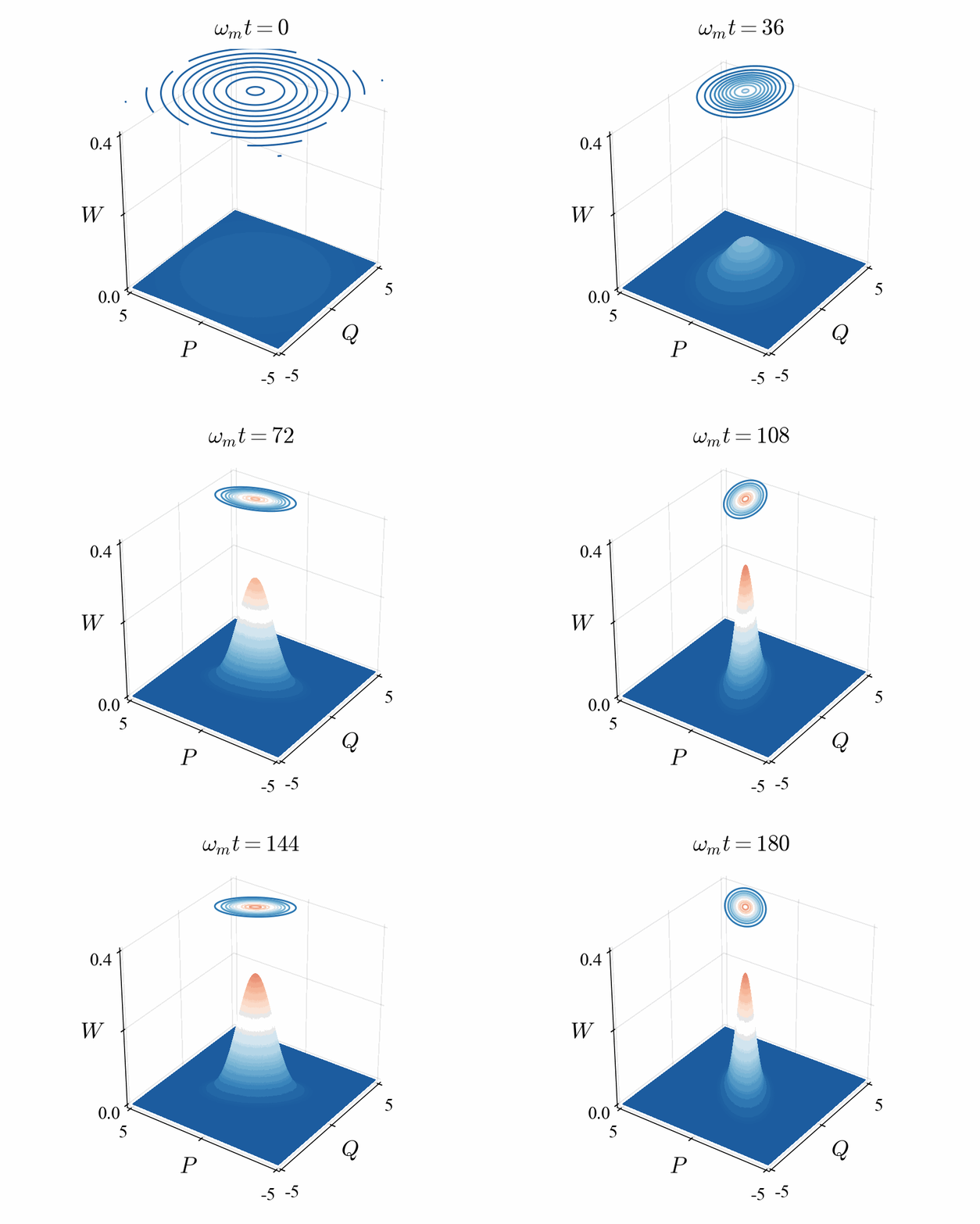
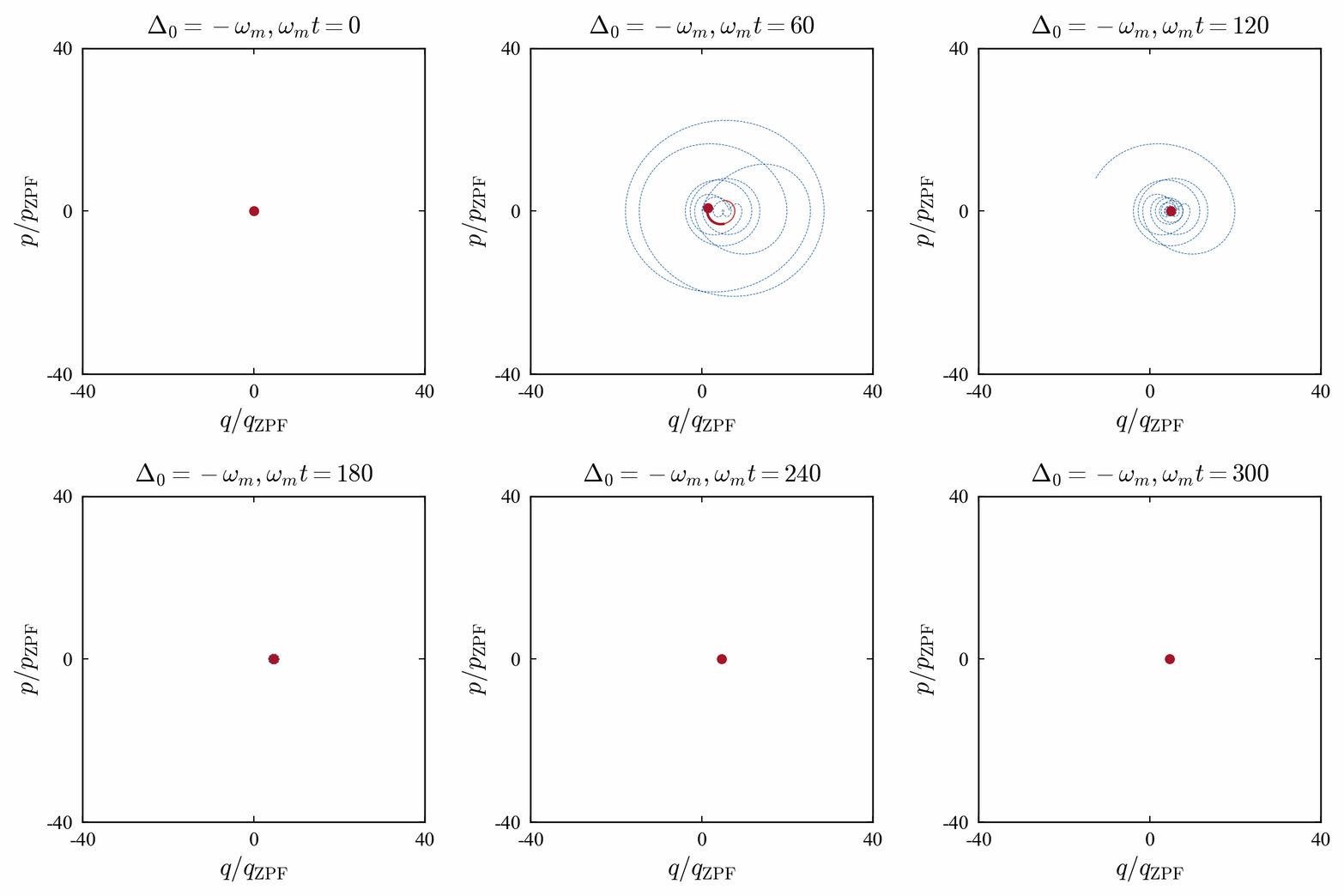
Fixed Point	Limit Cycle

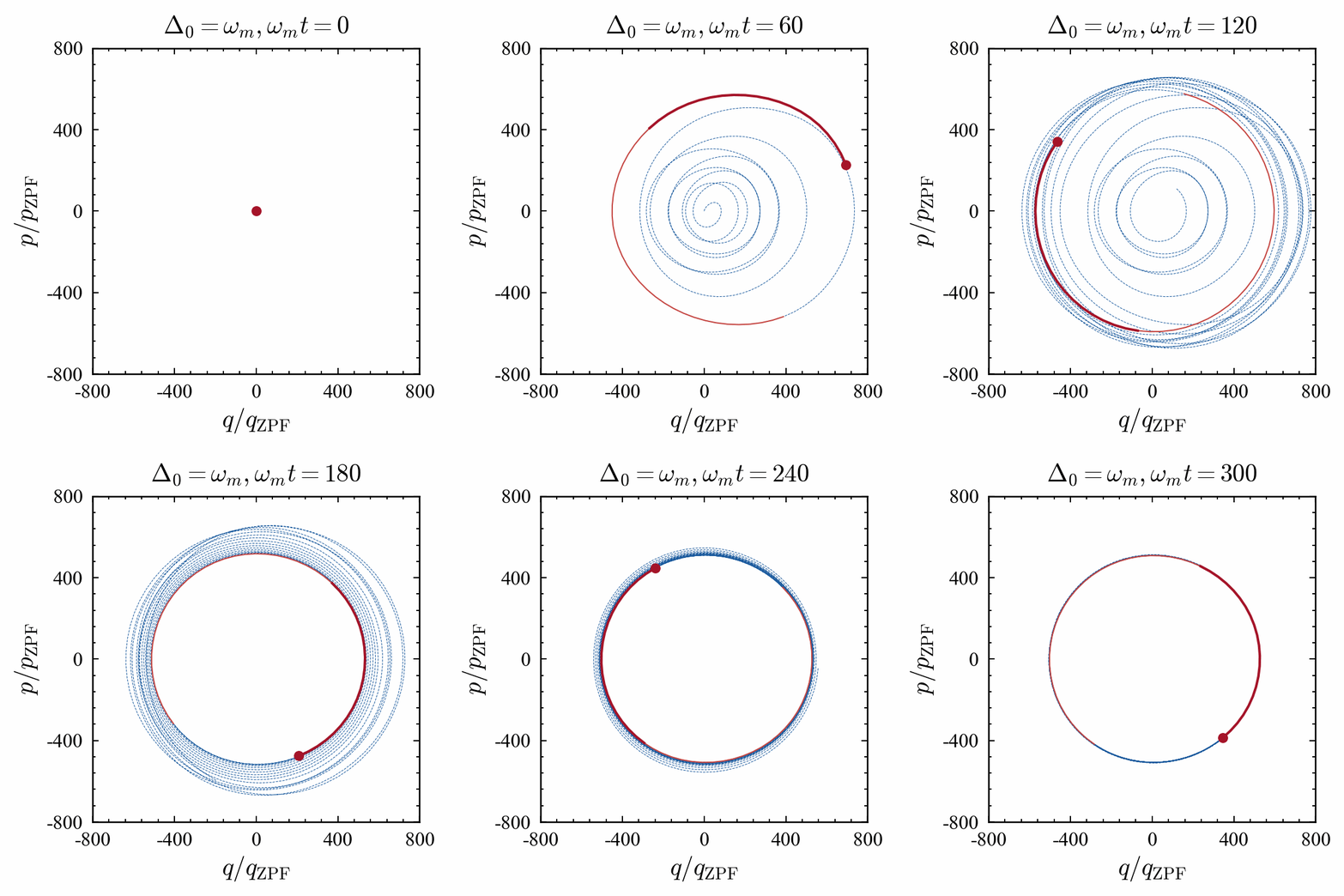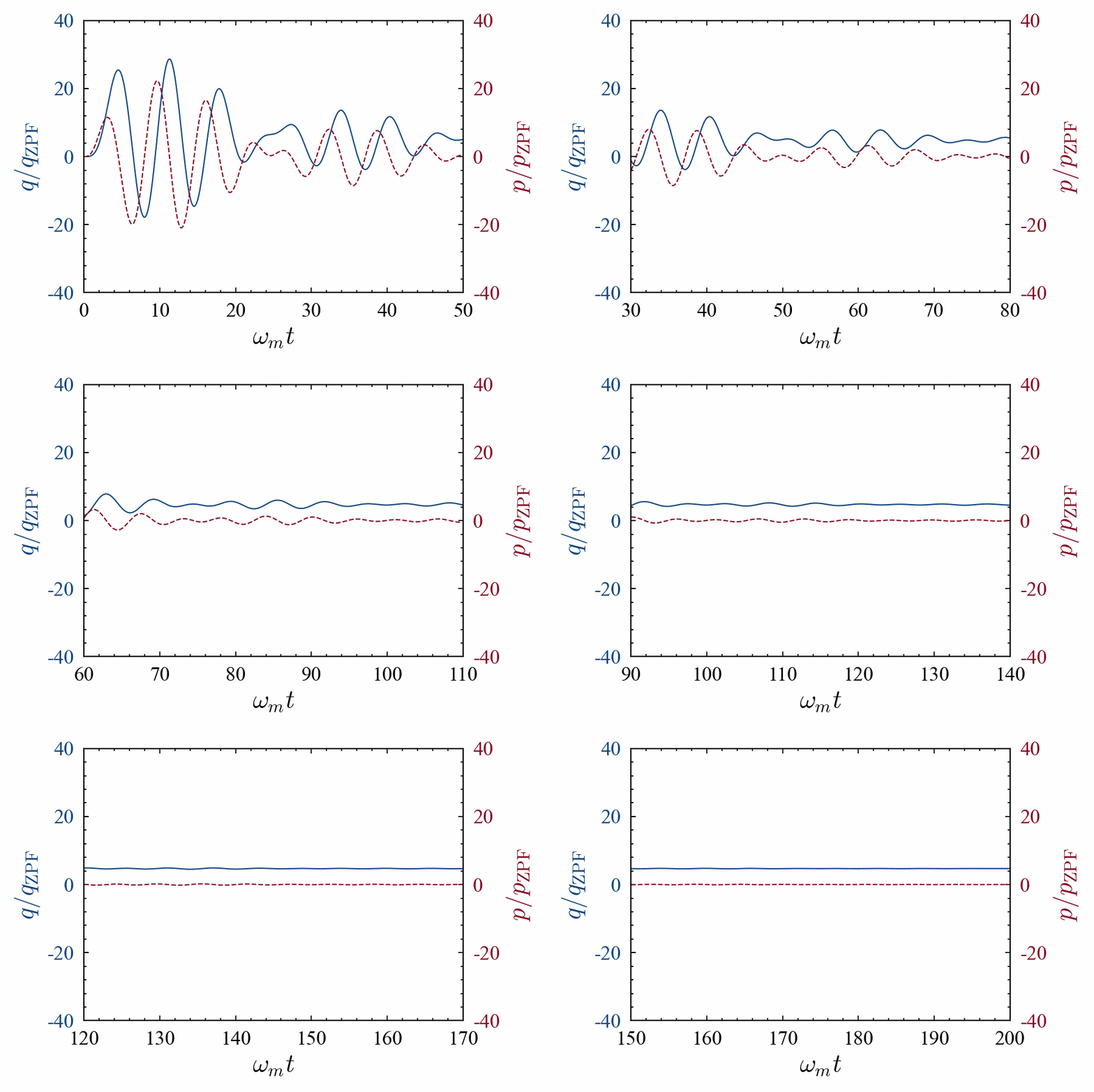
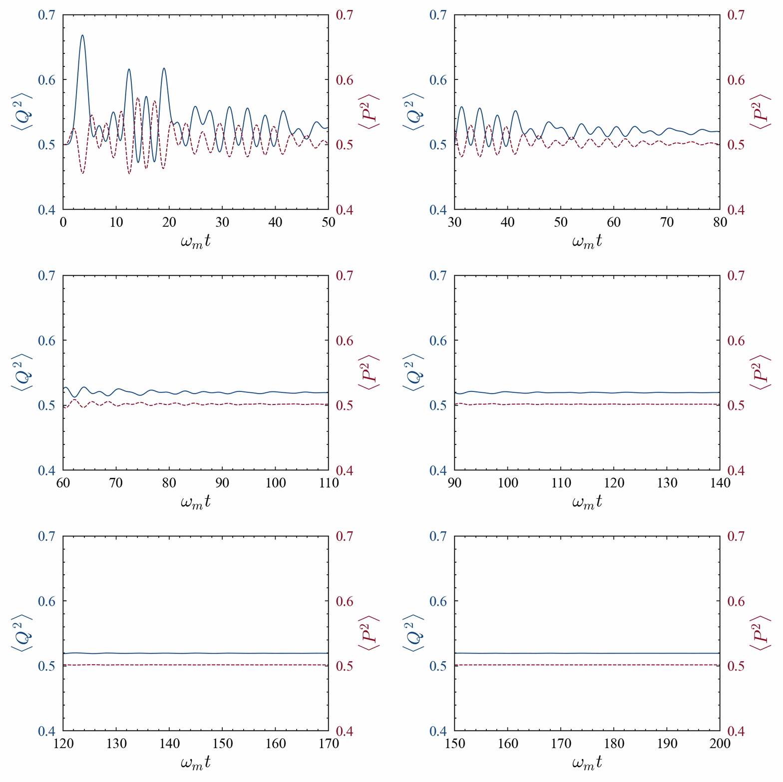
An optomechanical system settling to a steady state.	Self-sustained oscillations in an optomechanical system.

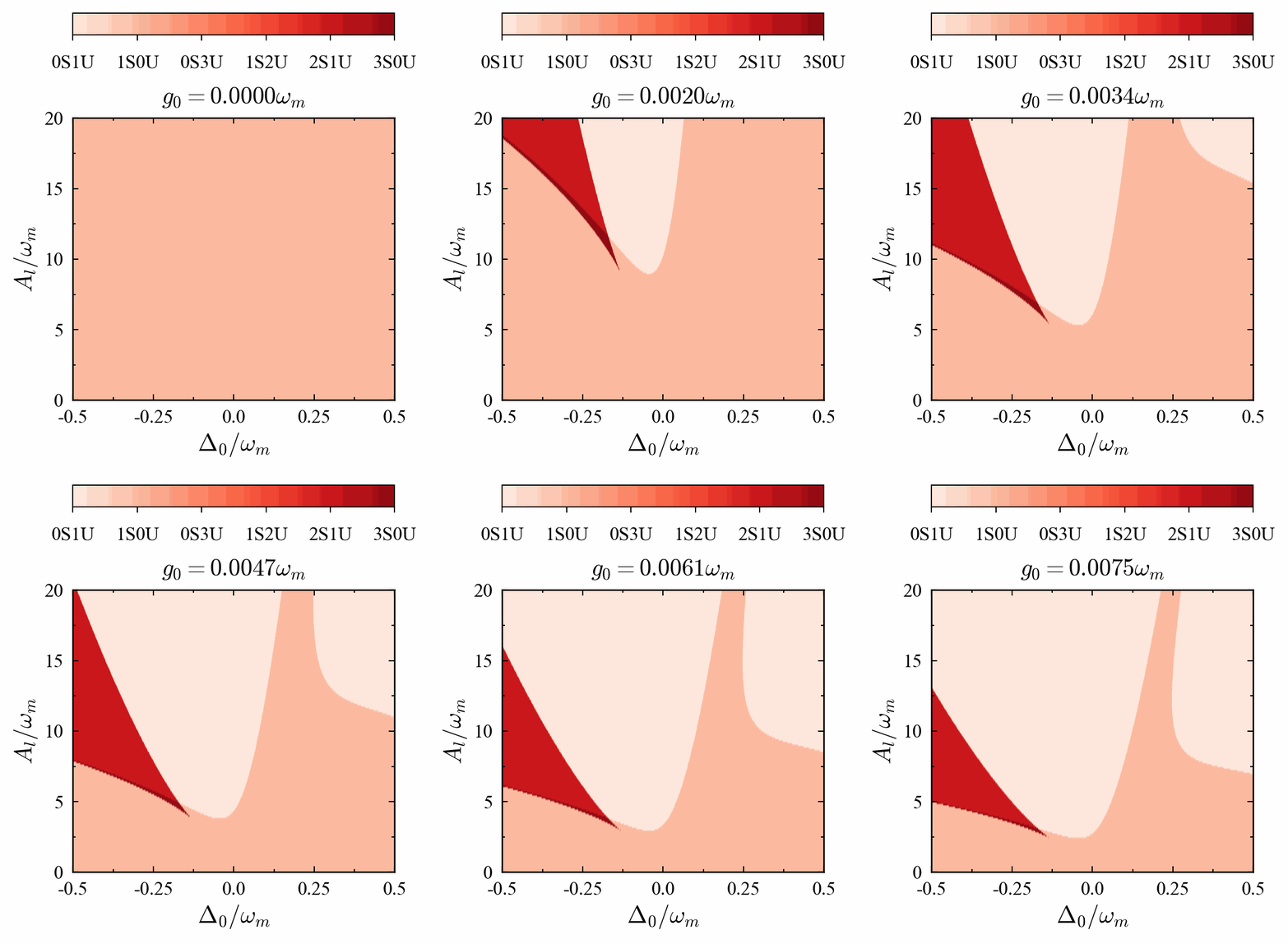
Dynamical Stability	Optical Bistability

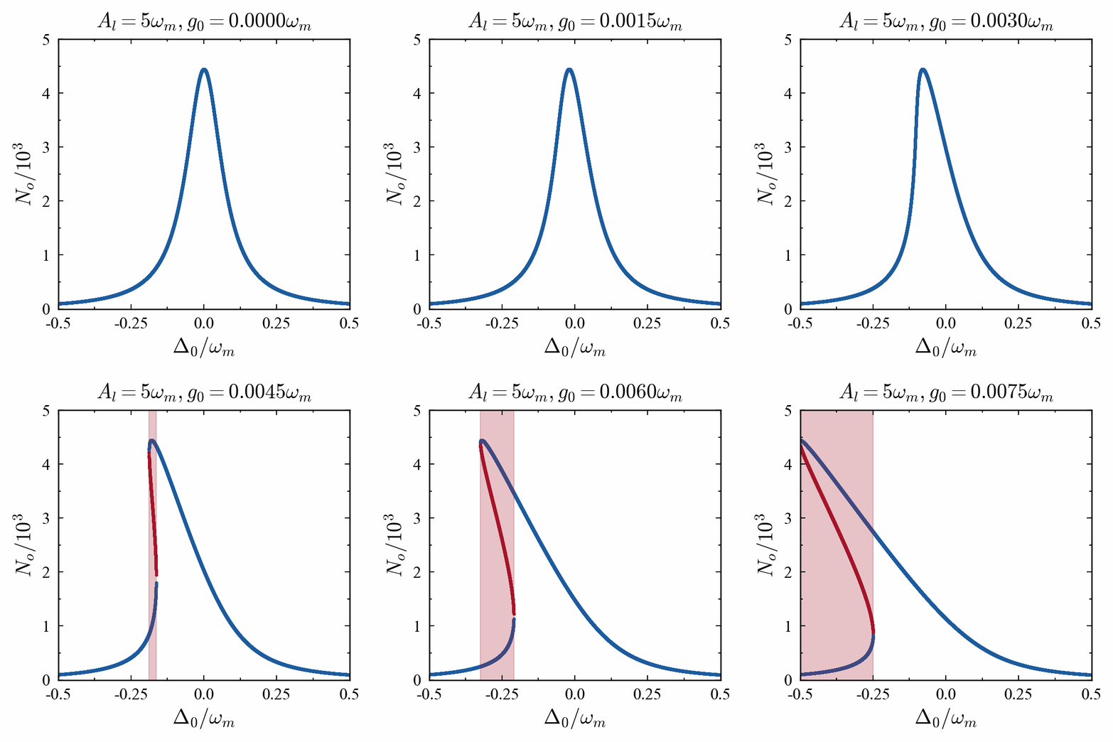Dynamical stability obtained from the steady state drift matrix.	Bistability obtained from the steady state optical occupancies.

Optomechanical Entanglement	Mechanical Synchronization

Quantum entanglement between the optical and mechanical modes of an optomechanical system.	Quantum phase synchronization between the mechanical modes of two coupled identical systems.

Wigner Distributions	Optomechanical Solitons

Wigner distribution depicting the evolution of mechanical squeezing in a modulated optomechanical system.	Soliton propagation in an array of optomechanical systems at different phase lags between the input solitons.

A set of notebooks and scripts to demonstrate the usage of the toolbox can be found in the examples repository.

Installation

Dependencies

The Quantum Optomechanics Toolbox requires Python 3.8+, preferably installed via the Anaconda distribution. Once Anaconda is set up, create and activate a new conda environment using:

conda create -n qom python
conda activate qom

The toolbox primarily relies on numpy (for fast numerical algebra), scipy (for numerical methods), sympy (for symbolic algebra), seaborn (for color palettes) and matplotlib (for plotting results). These libraries can be installed using:

conda install matplotlib numpy scipy sympy seaborn

Note: To run the GUI modules, pyqt should be installed separately.

Once the dependencies are installed, the toolbox can be installed via PyPI or locally.

The documentation of the latest release is available here.

Installing via PyPI

To install the last release via the Python Package Index, execute:

pip install git+https://github.com/sampreet/qom.git

Installing Locally

To install the latest version locally, download the repository as .zip and extract the contents. Now, execute the following from outside the top-level directory, ROOT_DIR, inside which setup.py is located (refer to the file structure):

pip install -e ROOT_DIR

Basic Usage

The library features easy-to-use functions to calculate as well as visualize the trend of several quantum signatures. A complete API documentation is available in the official website.

Loopers

The classes XLooper, XYLooper and XYZLooper loop over specific functions and parameters that are passed as arguments during initialization. The loop method returns the results in the form of a dictionary of the axes (X, Y and Z) and the calculated values V. The threshold values of the axes at which the calculations reach their minima or maxima can also be obtained using the get_thresholds method.

For example, the qom.looper.axes.XLooper class can be implemented as:

# initilize the looper with the function to loop and the looper parameters
looper = XLooper(func, params)
# get resultant dictionary containing keys `X` and `V`.
results = looper.loop()
# obtain the threshold values of the inputs
thres = looper.get_thresholds()

Here, func is a function containing the steps of each iteration and params is a dictionary containing the parameters of the looper. The complete documentation of the loopers is available here.

Solvers

Solvers constitute of a set of classes to tackle numerical computations of various forms. Each solver is associated with a particular method, measure or criterion.

For example, the qom.solvers.deterministic.HLESolver generates the time-varying solutions of the classical mode amplitudes and quantum correlations by solving the Heisenberg-Langevin equations and can be implemented as:

# initialize the solver with an instance of the system and solver parameters
solver = HLESolver(system, solver_params)
# solve for the dynamics of modes and correlations
Modes, Corrs = solver.get_modes_corrs()

Here, system is an instance of the user-defined system and solver_params is a dictionary containing the parameters of the solver. The complete documentation of the solvers is available here.

Systems

The BaseSystem class registers basic functionalities to streamline the solving and looping processes.

For example, the built-in function get_mean_optical_occupancies returns the intracavity photon numbers and can be implemented as:

# initialize the system with system parameters
system = MySystem(
    params=system_params
)
# obtain mean occupancy of the optical mode
N_os = system.get_mean_optical_occupancies()

Here, MySystem is a class inheriting BaseSystem, initialized by system_params, which is a dictionary containing the parameters of the system. The complete documentation of the BaseSystem class is available here.

UI

User-interface modules like qom.ui.log and qom.ui.gui provide console as well as graphical features to keep track of parameters and progress. Plotters wrap independent visualization packages of Python under an equivalent syntax. An implementation of qom.ui.plotters.MPLPlotter wrapping the matplotlib package is given below:

# initialize the plotter
plotter = MPLPlotter(
    axes={},
    params=plotter_params
)
# update the plot
plotter.update(
    vs=vs,
    xs=xs
)
# display the plot
plotter.show()

Utils

Utility functions provide an extra layer of ease over the other modules. The qom.utils.loopers module contains various functions that wrap loopers, together with an option to use plotter modules to visualize the results, thus trimming down several lines of code. Similarly, the qom.utils.solvers module contains various functions to quickly obtain dynamical or steady state properties and signatures.

For example, the qom.utils.loopers.wrap_looper function and the qom.utils.solvers.get_func_quantum_correlation_measures function can be utilized to cover everything in a single line of code:

# wrap looper and plot
wrap_looper(
    looper_name='XLooper',
    func=get_func_quantum_correlation_measures(
        SystemClass=MySystem,
        params=solver_params
    ),
    params=looper_params,
    params_system=system_params,
    plot=True,
    params_plotter=plotter_params
)

Alternatively, parallel instances of the loopers can be run using the qom.utils.loopers.run_loopers_in_parallel function.

Contributing

If you want to contribute to The Quantum Optomechanics Toolbox, check out the contribution guidelines. Also, make sure you adhere to the code of conduct.

Citing

Please cite S. Kalita and A. K. Sarma, The QOM Toolbox: An Object-oriented Python Framework for Cavity Optomechanical Systems, Proceedings of Eighth International Congress on Information and Communication Technology, Lecture Notes in Networks and Systems, Volume 694, 581-590, Springer Nature Singapore (2023) if you use our work in your research.

Sampreet/qom