TxGNN: Zero-shot prediction of therapeutic use with geometric deep learning and human centered design
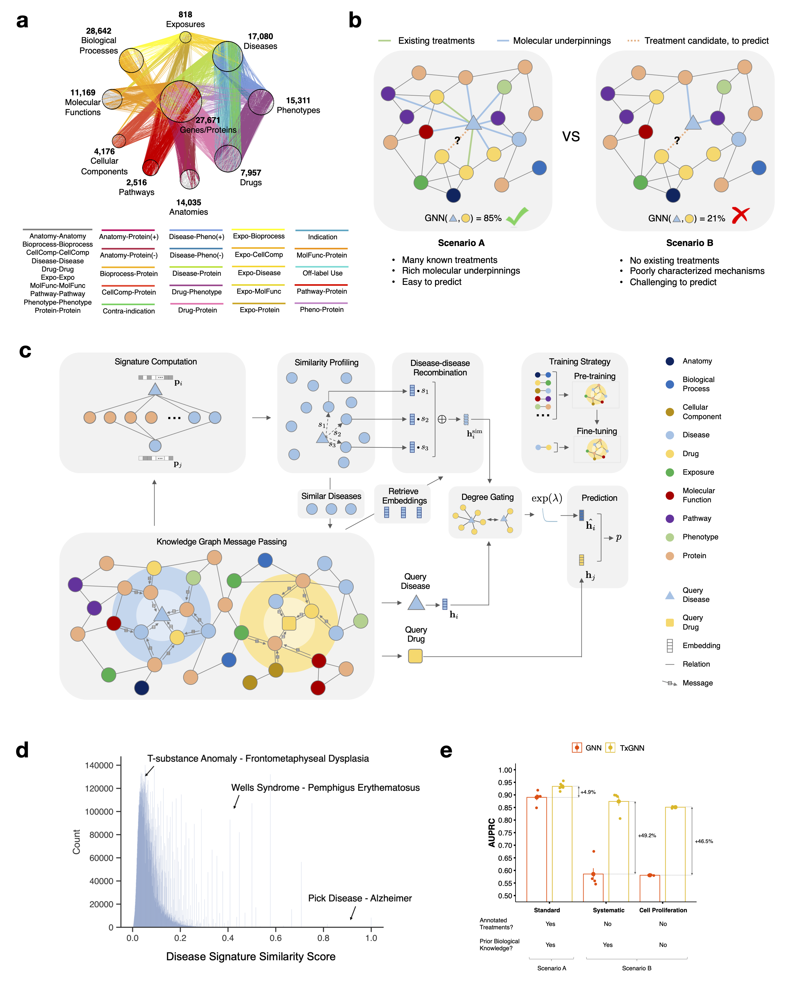
This repository hosts the official implementation of TxGNN, a model for identifying therapeutic opportunities for diseases with limited treatment options and minimal molecular understanding that leverages recent advances in geometric deep learning and human-centered.
TxGNN is a graph neural network pre-trained on a comprehensive knowledge graph of 17,080 clinically-recognized diseases and 7,957 therapeutic candidates. The model can process various therapeutic tasks, such as indication and contraindication prediction, in a unified formulation. Once trained, we show that TxGNN can perform zero-shot inference on new diseases without additional parameters or fine-tuning on ground truth labels.
MedRxiv preprint is at https://www.medrxiv.org/content/10.1101/2023.03.19.23287458
TxGNN Explorer of model predictions and explanations is at http://txgnn.org
conda create --name txgnn_env python=3.8
conda activate txgnn_env
# Install PyTorch via https://pytorch.org/ with your CUDA versions
conda install -c dglteam dgl-cuda{$CUDA_VERSION}==0.5.2 # checkout https://www.dgl.ai/pages/start.html for more info, as long as it is DGL 0.5.2
pip install TxGNN
Note that if you want to use disease-area split, you should also install PyG following this instruction since some legacy data processing code uses PyG utility functions.
Using the API, you can (1) reproduce the results in our paper and (2) train TxGNN on your own drug repurposing dataset using a few lines of code, and also generate graph explanations.
from txgnn import TxData, TxGNN, TxEval

# Download/load knowledge graph dataset
TxData = TxData(data_folder_path = './data')
TxData.prepare_split(split = 'complex_disease', seed = 42)
TxGNN = TxGNN(data = TxData,
              weight_bias_track = False,
              proj_name = 'TxGNN', # wandb project name
              exp_name = 'TxGNN', # wandb experiment name
              device = 'cuda:0' # define your cuda device
              )

# Initialize a new model
TxGNN.model_initialize(n_hid = 100, # number of hidden dimensions
                      n_inp = 100, # number of input dimensions
                      n_out = 100, # number of output dimensions
                      proto = True, # whether to use metric learning module
                      proto_num = 3, # number of similar diseases to retrieve for augmentation
                      attention = False, # use attention layer (if use graph XAI, we turn this to false)
                      sim_measure = 'all_nodes_profile', # disease signature, choose from ['all_nodes_profile', 'protein_profile', 'protein_random_walk']
                      agg_measure = 'rarity', # how to aggregate sim disease emb with target disease emb, choose from ['rarity', 'avg']
                      num_walks = 200, # for protein_random_walk sim_measure, define number of sampled walks
                      path_length = 2 # for protein_random_walk sim_measure, define path length
                      )
Instead of initializing a new model, you can also load a saved model:
TxGNN.load_pretrained('./model_ckpt')To do pre-training using link prediction for all edge types, you can type:
TxGNN.pretrain(n_epoch = 2,
               learning_rate = 1e-3,
               batch_size = 1024,
               train_print_per_n = 20)
Lastly, to do finetuning on drug-disease relation with metric learning, you can type:
TxGNN.finetune(n_epoch = 500,
               learning_rate = 5e-4,
               train_print_per_n = 5,
               valid_per_n = 20,
               save_name = finetune_result_path)
To save the trained model, you can type:
TxGNN.save_model('./model_ckpt')To evaluate the model on the entire test set using disease-centric evaluation, you can type:
from txgnn import TxEval
TxEval = TxEval(model = TxGNN)
result = TxEval.eval_disease_centric(disease_idxs = 'test_set',
                                     show_plot = False,
                                     verbose = True,
                                     save_result = True,
                                     return_raw = False,
                                     save_name = 'SAVE_PATH')
If you want to look at specific disease, you can also do:
result = TxEval.eval_disease_centric(disease_idxs = [9907.0, 12787.0],
                                     relation = 'indication',
                                     save_result = False)
After training a satisfying link prediction model, we can also train graph XAI model by:
TxGNN.train_graphmask(relation = 'indication',
                      learning_rate = 3e-4,
                      allowance = 0.005,
                      epochs_per_layer = 3,
                      penalty_scaling = 1,
                      valid_per_n = 20)
You can retrieve and save the graph XAI gates (whether or not an edge is important) into a pkl file located as SAVED_PATH/'graphmask_output_RELATION.pkl':
gates = TxGNN.retrieve_save_gates('SAVED_PATH')Of course, you can save and load graphmask model as well via:
TxGNN.save_graphmask_model('./graphmask_model_ckpt')
TxGNN.load_pretrained_graphmask('./graphmask_model_ckpt')There are numerous splits prepared in TxGNN. You can switch among them in the TxData.prepare_split(split = 'XXX', seed = 42) function.
complex_diseaseis the systematic split in the paper, where we first sample a set of diseases and then move all of their treatments to test set such that these diseases have zero treatments in training.- Disease area split first obtains a set of diseases in a disease area using disease ontology and move all of their treatments to the test set and then further removes a fraction of local neighborhood around these diseases to simulate the lack of molecular mechanism characterization of these diseases. There are five disease areas:
cell_proliferation,mental_health,cardiovascular,anemia,adrenal_gland randomis namely random splits which it randomly shuffles across drug-disease pairs. In the end, most of diseases have seen some treatments in the training set.
During deployment, when evaluate a specific disease, you may want to just mask this disease and use all of the other diseases. In this case, you can use TxData.prepare_split(split = 'disease_eval', disease_eval_idx = 'XX') where disease_eval_idx is the index of the disease of interest.
Another setting is to train the entire network without any disease masking. You can do that via split = 'full_graph'. This will automatically use 95% of data for training and 5% for validation set calculation to do early stopping. No test set is used.
@article{huang2023zeroshot,
  title={Zero-shot Prediction of Therapeutic Use with Geometric Deep Learning and Clinician Centered Design},
  author={Huang, Kexin and Chandak, Payal and Wang, Qianwen and Havaldar, Shreyas and Vaid, Akhil and Leskovec, Jure and Nadkarni, Girish and Glicksberg, Benjamin and Gehlenborg, Nils and Zitnik, Marinka},
  journal = {medRxiv},
  doi = {10.1101/2023.03.19.23287458},
  volume={},
  number={},
  pages={},
  year={2023},
  publisher={}
}
