SciCompDEV/OpenWavefrontReconstructor

Wavefront Reconstruction Algorithms

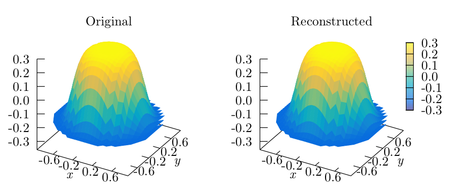
Open Wavefront Reconstructor: alfa

Note: version 1.0.0 will be uploaded soon

OWR (Open Wavefront Reconstructor) is a library written in C++ and aimed to facilitate future research in the field of wafefront reconstruction, as well as to provide a ready-to-go framework for being used in control systems.

The library contains the following capabilities:

• A mock-up generator of various types of incident wavefronts
• Implementation of different wavefront reconstruction algorithms: Zernike polynomials and Half Circular Harmonics for circular domains, and Legendre polynomials for square domains
• Runtime selection of the linear algebra library to perform the algebraic computations
• Time profiling of the linear algebraic operations

All software entities are fully decoupled, therefore OWR can be easily modified or extended.

Table of Contents

1. Introduction
2. Architecture
   1. Work Flow
   2. Uml
3. Installation
   1. Dependencies
   2. Build process and quick run
4. Usage
   1. Available runtime options through the custom parser
   2. MockUp generator
   3. Using external sensors
5. Contributing
6. FAQ

Introduction

A brief introduction to the mathematical background (intro+abstract of the paper), minimal number of equations. Reference to the paper

Architecture

Work Flow

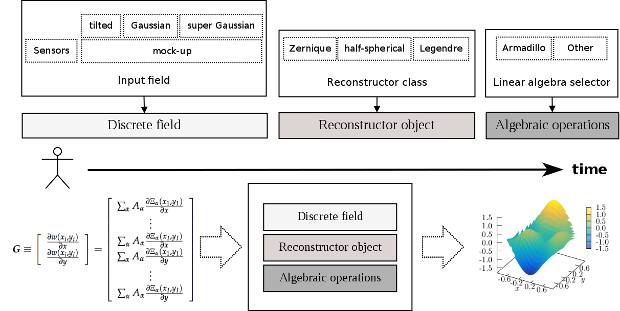
The diagram depicted below provides an overview of the different options offered by the library, and it shows a typical work flow that can be described as follows:

1. The user can choose the input wavefront as a simulated optical field generated by the mock-up generator, or as a direct input from a sensor. Usually, the sensor vendors provide libraries that can be used to retrieve information such as the focal spots coordinates, where the slopes are measured, and obviously these also provide the slopes. These coordinates and slopes are the inputs received by OpenWavefrontReconstructor, and are used to configure the matrices M and R defined by Equations (8) and (11).
2. Similarly, the user can choose the particular algorithm that will perform the wavefront reconstruction, which can be instantiated as an object from the available classes representing the different approaches (see the previous enumeration list—item 2—for the list of available polynomials).
3. Finally, the user can also select, at runtime, the linear algebra library to perform the linear algebraic operations.

Note: in version 1.0.0 of OWR, only the armadillo library is merged in the code; however, we plan to include more options, and the user can also implement the libraries of his/her preference. OWR's design is intended to provide an easy-to-follow (nearly copy-paste) environment to implement new linear algebra libraries.

Uml

Sequence and class diagrams are (will be) included in doc folder:

sequenceDiagram.odg
UML.xmi

Installation

Dependencies

• The algebraic operations are implemented by means of the linear algebra library armadillo.
• The logging is performed by log4CXX.
• To 3D plot the final graphics the command-line driven graphing utility Gnuplot.

Build process and quick run

To generate the executable in SRC/bin:

cd SRC
make all

And to execute it:

cd SRC/bin
./OWR

Note that in the same folder bin are located:

• the configuration file for the logging facility: Log4cxxConfig.xml
• the parser file with the available runtime options: config.cfg

Usage

Available runtime options through the custom parser

The OWR executable

Parser var name	Implemented options	Description
libtype	armadillo	The linear algebra library
mock_type_wavefront	Circular CircularTestF1 CircularXYTilted CircularCenteredGaussian CircularOffCenteredGaussian CircularDoubleOffCenteredGaussians CircularSuperGaussian4 CircularSuperGaussian6 CircularSuperGaussian8 Square SquareXYTilted SquareTestF1 SquareCenteredGaussian SquareOffCenteredGaussian SquareDoubleOffCenteredGaussians SquareSuperGaussian4 SquareSuperGaussian6 SquareSuperGaussian8	Shape of simulated optical field (surface)
polynomialbasis	Zernike HalfCircularHarmonics Legendre	The polynomial set used for reconstructing the wavefront. By default, Zernike and HalfCircularHarmonics assume that the wavefront is defined on a circle. Legendre, on the other hand, assumes that the wavefront is defined on a square.
polynomialorder	An integer. Tested values: 4 to 12 for HalfCircularHarmonics 6 to 17 for Zernike However, there should be no restrictions as to this number, other than memory restraints.	Principal order of the polynomial set

MockUp generator

The library includes a wavefront generator (the class MockWaveFrontGenerator provides both the surface as well as the gradients of the surface; the surface and gradients are evaluated aa a set of points, which are also generated by the MockWaveFrontGenerator object). The shapes of the wavefronts are listed above (as options for the mock_wave_front keyword).

Custom gradients can also be parsed. Should you like support on this, please read the Contributing section on how to get support.

Using external sensors

If you'd like to see support for using the library within your custom wavefront sensor software, please create an issue or create a pull request. If you'd like to discuss the project more directly, feel free to reach us out through the emails in the SciCompDEV organizational repository.

Contributing

If you'd like to see support for more options, please create an issue or create a pull request. If you'd like to discuss the project more directly, feel free to reach us out through the emails in the SciCompDEV organizational repository.

FAQ

Known bugs/limitations

The point (x,y)=(0,0) must not be present in the grid, because this point causes some problems in the reconstruction. To the best of our knowledge this problem is also present in the Zernike reconstruction. A good strategy is to remove it from the grid, and the best is to set of the center of the grid such that the first neighbor nodes are +-l/2 (in both x and y directions), where l is the distance between two consecutive nodes either in x or y direction.