The coevolve package allows the user to fit Bayesian dynamic coevolutionary phylogenetic models in Stan. These models can be used to estimate how variables have coevolved over evolutionary time and to assess causal directionality (X → Y vs. Y → X) and contingencies (X, then Y) in evolution.
While existing methods only allow pairs of binary traits to coevolve (e.g., BayesTraits), the coevolve package allows users to include multiple traits of different data types, including binary, ordinal, count, and continuous traits.
To use the coevolve package, you must first install the cmdstanr
package (see full installation instructions here:
https://mc-stan.org/cmdstanr/).
install.packages("cmdstanr", repos = c("https://mc-stan.org/r-packages/", getOption("repos")))You can then install the development version of coevolve with:
# install.packages("devtools")
devtools::install_github("ScottClaessens/coevolve")library(coevolve)As an example, we analyse the coevolution of political and religious authority in 97 Austronesian societies. These data were compiled and analysed in Sheehan et al. (2023). Both variables are four-level ordinal variables reflecting increasing levels of authority. We use a phylogeny of Austronesian languages to assess patterns of coevolution.
fit <-
  coev_fit(
    data = authority$data,
    variables = list(
      political_authority = "ordered_logistic",
      religious_authority = "ordered_logistic"
    ),
    id = "language",
    tree = authority$phylogeny,
    # manually set prior
    prior = list(A_offdiag = "normal(0, 2)"),
    # arguments for cmdstanr
    parallel_chains = 4,
    iter_sampling = 500,
    refresh = 0,
    seed = 1
  )
#> Running MCMC with 4 parallel chains...
#>
#> Chain 4 finished in 1165.9 seconds.
#> Chain 3 finished in 1551.9 seconds.
#> Chain 2 finished in 1591.5 seconds.
#> Chain 1 finished in 1601.1 seconds.
#>
#> All 4 chains finished successfully.
#> Mean chain execution time: 1477.6 seconds.
#> Total execution time: 1601.3 seconds.
#> Warning: 61 of 2000 (3.0%) transitions ended with a divergence.
#> See https://mc-stan.org/misc/warnings for details.
The results can be investigated using:
summary(fit)
#> Variables: political_authority = ordered_logistic
#>            religious_authority = ordered_logistic
#>      Data: authority$data (Number of observations: 97)
#>     Draws: 4 chains, each with iter = 500; warmup = 1000; thin = 1
#>            total post-warmup draws = 2000
#>
#> Autoregressive selection effects:
#>                     Estimate Est.Error  2.5% 97.5% Rhat Bulk_ESS Tail_ESS
#> political_authority    -0.61      0.51 -1.91 -0.03 1.01     1589      964
#> religious_authority    -0.68      0.53 -1.98 -0.03 1.01     1170      665
#>
#> Cross selection effects:
#>                                           Estimate Est.Error 2.5% 97.5% Rhat
#> political_authority ⟶ religious_authority     2.99      1.20 0.84  5.58 1.02
#> religious_authority ⟶ political_authority     2.43      1.08 0.65  4.88 1.01
#>                                           Bulk_ESS Tail_ESS
#> political_authority ⟶ religious_authority      189       74
#> religious_authority ⟶ political_authority      666      833
#>
#> Drift scale parameters:
#>                     Estimate Est.Error 2.5% 97.5% Rhat Bulk_ESS Tail_ESS
#> political_authority     1.52      0.74 0.23  3.05 1.01      772      685
#> religious_authority     1.18      0.71 0.09  2.72 1.01      668      972
#>
#> Continuous time intercept parameters:
#>                     Estimate Est.Error  2.5% 97.5% Rhat Bulk_ESS Tail_ESS
#> political_authority     0.14      0.93 -1.61  1.91 1.01     2427     1288
#> religious_authority     0.15      0.91 -1.69  1.93 1.01     2063     1300
#>
#> Ordinal cutpoint parameters:
#>                        Estimate Est.Error  2.5% 97.5% Rhat Bulk_ESS Tail_ESS
#> political_authority[1]    -1.03      0.84 -2.67  0.73 1.00     1590     1088
#> political_authority[2]    -0.33      0.83 -1.95  1.42 1.00     1693     1288
#> political_authority[3]     1.63      0.86  0.02  3.40 1.01     1640     1397
#> religious_authority[1]    -1.32      0.87 -3.00  0.35 1.00     1428     1415
#> religious_authority[2]    -0.68      0.84 -2.23  0.94 1.00     1479     1532
#> religious_authority[3]     1.64      0.92 -0.09  3.44 1.01      770      714
#> Warning: There were 61 divergent transitions after warmup.
#> http://mc-stan.org/misc/warnings.html#divergent-transitions-after-warmup
The summary provides general information about the model and details on the posterior draws for the model parameters. In particular, the output shows the autoregressive selection effects (i.e., the effect of a variable on itself in the future), the cross selection effects (i.e., the effect of a variable on another variable in the future), the amount of drift, continuous time intercept parameters for the schocastic differential equation, and cutpoints for the ordinal variables.
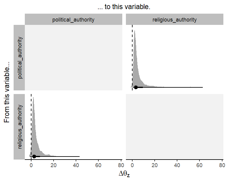
While this summary output is useful as a first glance, it is difficult to interpret these parameters directly to infer directions of coevolution. Another approach is to “intervene” in the system. We can hold variables of interest at their average values and then increase one variable by a standardised amount to see how this affects the optimal trait value for another variable.
The coev_plot_delta_theta() function allows us to visualise
coev_plot_delta_theta(fit)This plot suggests that both variables influence one another in their coevolution. A standardised increase in political authority results in an increase in the optimal trait value for religious authority, and vice versa. In other words, these two variables reciprocally coevolve over evolutionary time.
When using the coevolve package, please cite the following papers:
- Ringen, E., Martin, J. S., & Jaeggi, A. (2021). Novel phylogenetic methods reveal that resource-use intensification drives the evolution of “complex” societies. EcoEvoRXiv. https://doi.org/10.32942/osf.io/wfp95
- Sheehan, O., Watts, J., Gray, R. D., Bulbulia, J., Claessens, S., Ringen, E. J., & Atkinson, Q. D. (2023). Coevolution of religious and political authority in Austronesian societies. Nature Human Behaviour, 7(1), 38-45. https://doi.org/10.1038/s41562-022-01471-y


