Practical : Strain resolution

Plan for the session:

learn how to launch the STRONG pipeline
learn the main step of the analysis, and it's expected output
(time dependant) introduction to snakemake and how to create your own pipeline

STRONG - Strain Resolution ON Graphs

Overview

The STRONG pipeline can be subdivided in these 4 main steps. Steps

assembly: coassembly of sample, binning, MAG assessment
graphextraction: extract cogs subgraphs
bayespaths: Use bayespaths to infer strains and coverage
results: Generate results figures.

STRONG resolves strains on assembly graphs by resolving variants on core COGs using co-occurrence across multiple samples.

Before starting

Installation

STRONG is already installed on your VM, you will find the git repos at: ~/repos/STRONG It is a clone of the one available online and installation steps are detailed there.

Packages needed: Current installation depend entirely on conda, by creating an environment where all packages and their dependencies are installed.

Look at : ~/repos/STRONG/conda_env.yaml

fasttree is a dependency, it has been installed, try :

fasttree -h

not working?

Try activating the relevant conda environment :

conda env list
conda activate STRONG
fasttree -h

Databases

COG database , you will find it installed at /home/training/Databases/rpsblast_cog_db
(optional) GTDB , used with gtdb-tk, (77Gb) too much ram needed and execution too slow for this present tutorial.

Dataset

Anaerobic digester metagenomic time series subsampled for this tutorial, reads mapping only to a few bins of interest. Please download and extract the dataset using this link:

mkdir ~/Data 
cd ~/Data
wget http://seb.s3.climb.ac.uk/strain_practial_data.tar.gz
tar -xvf strain_practial_data.tar.gz

Look inside a read file with nano, less, head, tail, more or any such:

How to count the number of reads?

echo $(cat ~/Data/AD_small/sample1/sample1_R1.fastq | wc -l )/4| bc

Can you understand what each program does here, cat, wc, bc?

while not exhaustive, have a look at cheatsheets for bash commands , or bash scripting.

Additional files

Please download this repos which contains some intermediary results, scripts and files needed for this session.

cd ~/repos
git clone https://github.com/Sebastien-Raguideau/strain_resolution_practical.git

Some part of STRONG are a bit too slow and we will have to work with pre-run results. Please download and extract theses files:

cd ~/repos/strain_resolution_practical
wget http://seb.s3.climb.ac.uk/STRONG_prerun.tar.gz
tar -xvf STRONG_prerun.tar.gz

Launching STRONG : config file

To use STRONG, you need to create a config file which is used to store the parameters of a run. It is divided into sections with parts corresponding to the different steps of the pipeline.

Let's create a working directory, and copy the config file template:

mkdir -p ~/Projects/STRONG_AD
cd ~/Projects/STRONG_AD
cp ~/repos/strain_resolution_practical/config_template.yaml config.yaml

Look at the config.yaml with more:

more config.yaml

For 5-10 mins try to use the STRONG documentation to fill in this config file. Edit the config file with nano or vi so that it runs the samples in:

 /home/training/Data/AD_small

Check that your config file works with the dryrun command.

cd  ~/Projects/STRONG_AD
rm -r STRONG_OUT
STRONG --config config.yaml STRONG_OUT assembly --threads 8 --dryrun --verbose

Is something wrong with your config file?

Debuging a config file:

First it has to be a valid .yaml file, here is the format definition and here is a validator. In short, don't forget indentations or colons.
you only have 2 paths to fill the path to the sample folder and the path to the cog database. If you have issues, you may have mispellled any of these. Use the ls command to check the path exists.
the cog database path is /home/training/Databases/rpsblast_cog_db
the data folder path is: /home/training/Data/AD_small

It's still not working?

Well, we can't spend too long on debugging everybody, just copy and paste the correct config file from the strain_practical repo.

cd ~/Projects/STRONG_AD
cp  ~/repos/strain_resolution_practical/config_correct.yaml config.yaml

When using the dryrun option what happens?

Assembly

Let's launch STRONG for real this time:

cd ~/Projects/STRONG_AD
rm -r STRONG_OUT
STRONG --config config.yaml STRONG_OUT assembly --threads 8

We only started running the first step of STRONG, the assembly step, it consists of more than 150 tasks

This should take about twenty minutes. We are not waiting for that instead kill the strong run using Ctrl-C and copy in the prerun assembly after cleaning up the output directory:

    cd ~/Projects/STRONG_AD
    rm -r -f STRONG_OUT
    mkdir STRONG_OUT
    cp -r ~/repos/strain_resolution_practical/STRONG_prerun/assembly ~/Projects/STRONG_AD/STRONG_OUT

The restart the assembly step:

    STRONG --config config.yaml STRONG_OUT assembly --threads 8

Whilst that is running login on a separate terminal so we can look at the assembly output - don't forget to restart the STRONG conda environment:

Coassembly

cd  ~/Projects/STRONG_AD/STRONG_OUT/
ls -lh assembly/spades/contigs.fasta

How good is the coassembly, what is the N50? What is a good coassembly? Btw, why a coassembly? when a coassembly?

~/repos/strain_resolution_practical/scripts/contig-stats.pl < ./assembly/spades/contigs.fasta

sequence #: 1966 total length: 6377796 max length: 174676 N50: 28942 N90: 3000

Assembly graph

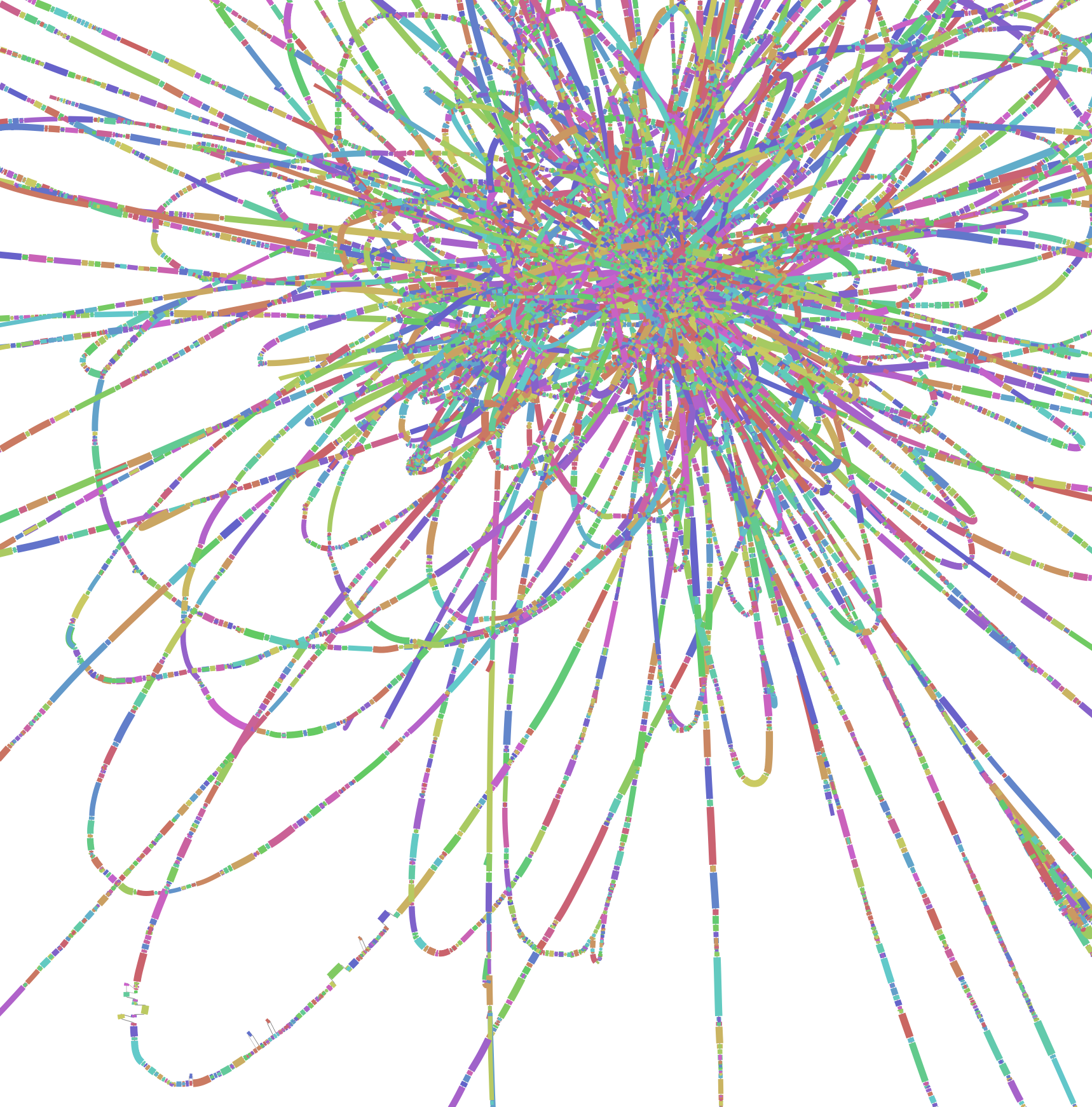
Other useful things to look at include the simplified graph that will be used for strain resolution. This can be visualised with Ryan Wick's excellent Bandage program:

ls -l -h assembly/high_res/simplified.gfa

Why do we use a "high resolution assembly graph"?

Lets take some time to look at the assembly graph with bandage

 Bandage load assembly/high_res/simplified.gfa`

Using Bandage it is possible to extract part of the assembly graph with a command such as

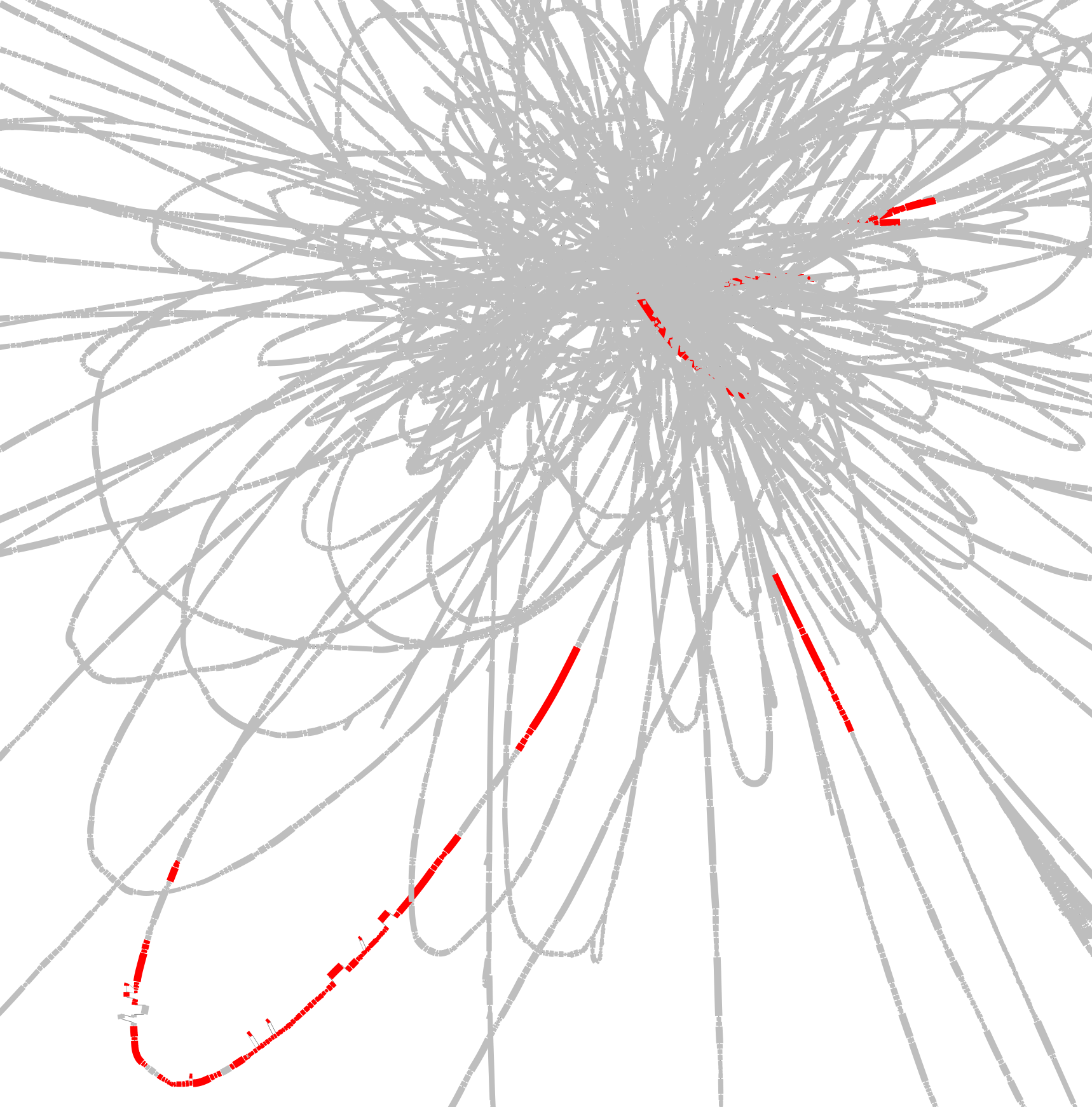
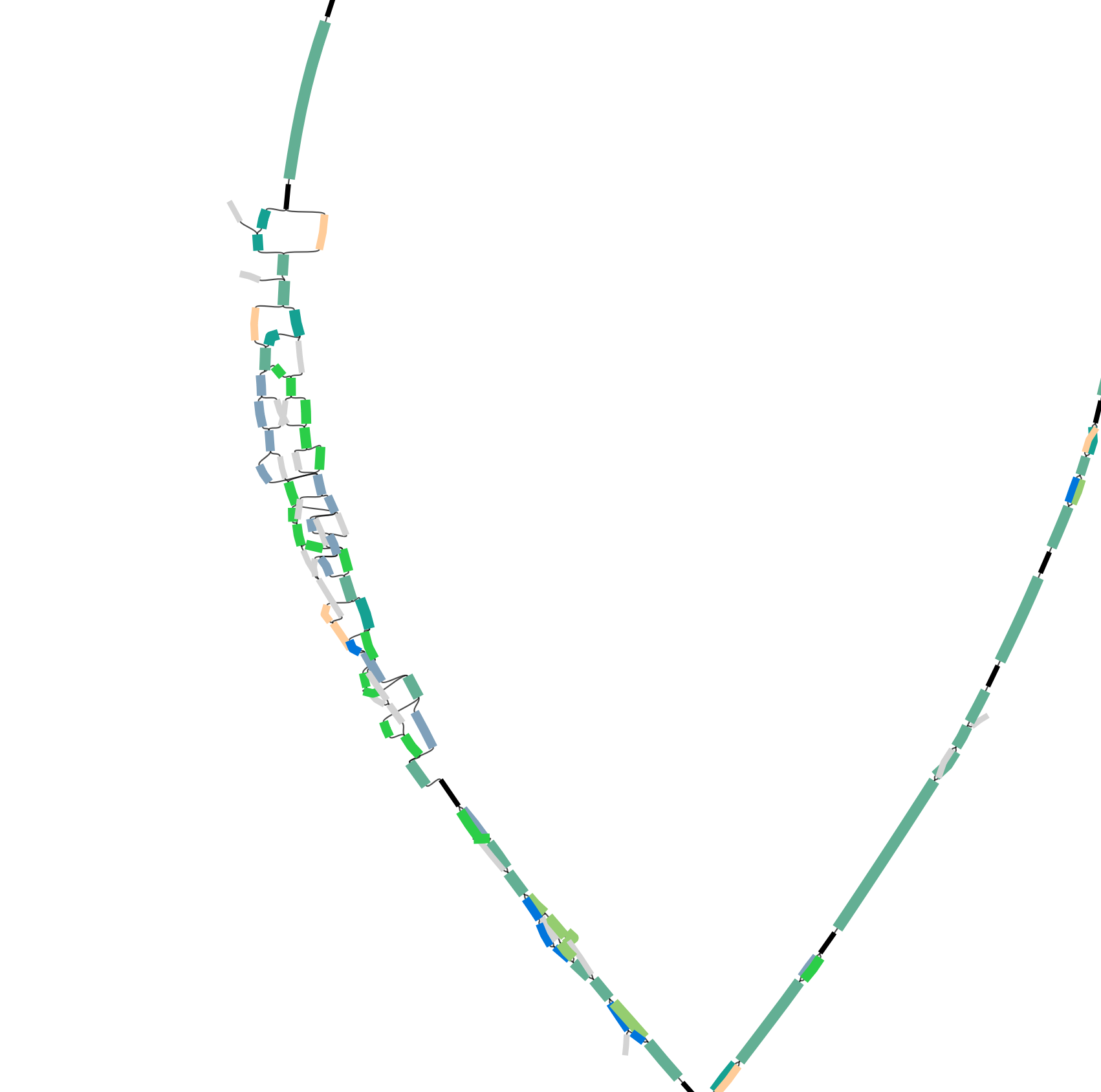
 Bandage reduce <INPUT_GRAPH.gfa>  <NAME_OF_OUTPUT.gfa> --scope aroundnodes --nodes <NODE> --distance 0

I did that for the exact same COG0016 from 3 assembly graph files:

on assembly/spades/assembly_graph_with_scaffolds.gfa
on assembly/high_res/graph_pack.gfa
on assembly/high_res/simplified.gfa

Open and visualise the "simplified" assembly graph:

What are the differences between the 3 assemblies graph? Can you tell which sequence comes from which type of assembly?

On the normal assembly we can see a unique contig, but in reality there are 3 strains. Why is there only 1 contigs?

unitig multi sample coverage profile

And the unitig per sample profiles, these are generated by thread threading reads onto the simplified graph, Sergey Nurk's application unitig-coverage does this:

tail assembly/high_res/simplified.mult_prof

Hopefully the assembly step should have finished by now so we can look at the binning output

binning

This step of the pipeline also does bowtie2 mapping of reads onto contigs to get coverage profiles for binning:

cd ~/Projects/STRONG_AD/STRONG_OUT
head profile/split/coverage.tsv

It also does the actual binning using by default a two step version of CONCOCT although metabat2 is an option:

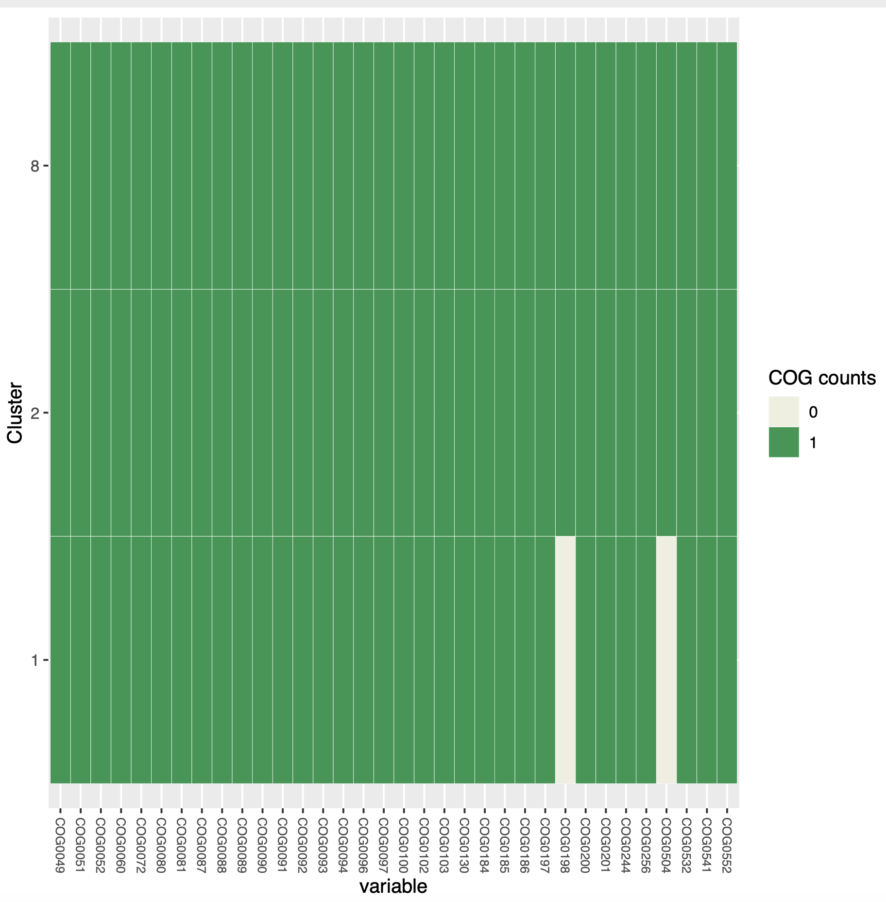
more binning/concoct/list_mags.tsv

There should be three MAGs generated for the next steps in the analysis. Can look at SCG frequencies in MAGs:

cd binning/concoct/
tr "," "\t" < SCG_table_concoct.csv > SCG_table_concoct.tsv
cp ~/repos/strain_resolution_practical/scripts/COGPlot.R .
Rscript ./COGPlot.R -s SCG_table_concoct.tsv -o SCG_table_concoct.pdf

Can visualise with evince if you have X-windows forwarding and logged on with ssh -Y:

evince SCG_table_concoct.pdf

Subgraph Extraction

The next step is to extract out and simplify the SCG subgraphs for the actual bayespaths strain finding. We run this as above just change assembly to graphextraction:

cd ~/Projects/STRONG_AD
STRONG --config config.yaml STRONG_OUT graphextraction --threads 8 --verbose

Which are again in gfa format with coverages.

Raw subgraph: subgraph directly taken from assembly/high_res/simplified.gfa
simplified subgraph: Raw subgraph further processed "simplified" using coverage. These subgraph do not match the initial assembly graph.

BayesPaths

These steps generate all the input required for the strain resolving algorithm BayesPaths. As it takes about 20~30 min to run automatically, let's launch it now.

cd ~/Projects/STRONG_AD
STRONG --config config.yaml STRONG_OUT bayespaths --threads 8 --verbose

Manual version

Whilst we wait for that login on a separate terminal (don't forget to reactivate STRONG) and do a few trial runs to better understand the inputs first. Let's test out the most complex bin Bin_2 in my run:

cd ~/Projects/STRONG_AD/STRONG_OUT/subgraphs/bin_merged
wc Bin_*/simplif/*0060*tsv

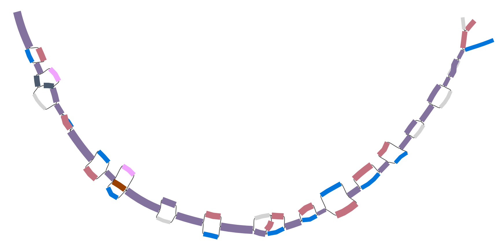
COG0060 for this MAG looks like:

Can look at the results which are again in gfa format:

Then visualise the simplified COG gfa in bandage:

Bandage load Bin_2/simplif/COG0060.gfa

Can you find and load the raw graph next - is there any difference?

We might estimate this contains three strains, can we confirm that. We will do a trial run of BayesPaths to test this, in a new directory:

cd ~/Projects/STRONG_AD/STRONG_OUT
mkdir BPTest
cd BPTest

Then we will run BayesPaths with a minimum number of NMF iterations and the gene filtering disabled. Type bayespaths for usage.

usage: bayespaths [-h] [-l [COG_LIST]] [-t [LENGTH_LIST]] [-f [FRAC_COV]]
                  [-m [MIN_COV]] [-mf [MIN_FRAC_COV]] [-g [STRAIN_NUMBER]]
                  [--loess] [--no_gam] [--no_ard] [--no_noise] [-i ITERS]
                  [-nfo NOFOLDS] [-r [READLENGTH]] [-s RANDOM_SEED]
                  [-e [EXECUTABLE_PATH]] [-u [UNCERTAIN_FACTOR]]
                  [-nr NMF_ITERS] [-ngf MAX_GITER] [--noscale_nmf]
                  [--nofilter] [--norun_elbow] [--norelax] [--nobias]
                  [--bias_type {unitig,gene,bubble}]
                  [--tau_type {fixed,log,empirical,auto,poisson}]
                  [--nogenedev]
                  Gene_dir kmer_length outFileStub
bayespaths: error: the following arguments are required: Gene_dir, kmer_length, outFileStub

Then run:

ln -s ../subgraphs/bin_merged/Bin_2 Bin_2
cp ~/repos/STRONG/BayesPaths/Data/coreCogs.tsv .

and finally bayespaths itself:

bayespaths Bin_2/simplif 77 Bin_2 -r 150 -l Bin_2/selected_cogs.tsv -t coreCogs.tsv -g 4 --nofilter -nr 1 -e ~/repos/STRONG/BayesPaths/runfg_source/

This will take a little time. It should select three strains. We can have a look at the output:

If it takes too long on your VM have a look at the prerun results:

cd ~/repos/strain_resolution_practical/STRONG_prerun/bayespaths/Bin_2

Otherwise stay in this dir.

Then let's look at the output files:

Bin_2F_Pred.csv

Bin_2F_Pred.csv contains coverage of unitigs as well as coverage from strain contributions.

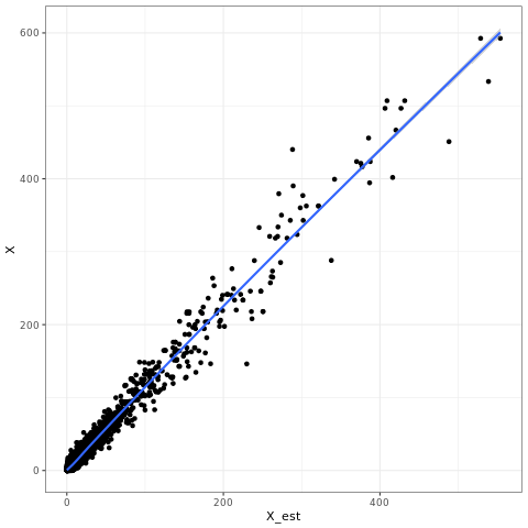
Let's generate a simple plot of fit:

R
Pred <- read.csv('Bin_2F_Pred.csv',header=T)
library(ggplot2)
pdf('X.pdf')
qplot(data=Pred,x=X_est,y=X) + geom_smooth() + theme_bw()
dev.off()
q()

Then visualise plot:

evince X.pdf

Bin_2F_maxPath.tsv

grep "COG0060" Bin_2F_maxPath.tsv | sed 's/COG0060_//g' > Bin_2F_maxPath_COG0060.tsv
python ~/repos/STRONG/BayesPaths/scripts/Add_color.py ../../subgraphs/bin_merged/Bin_2/simplif/COG0060.gfa Bin_2F_maxPath_COG0060.tsv > COG0060_color.gfa

This can be visualised in Bandage on your local machine may be easier

Bandage load COG0060_color.gfa

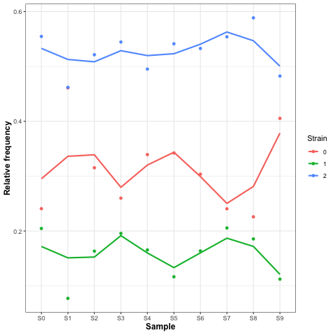
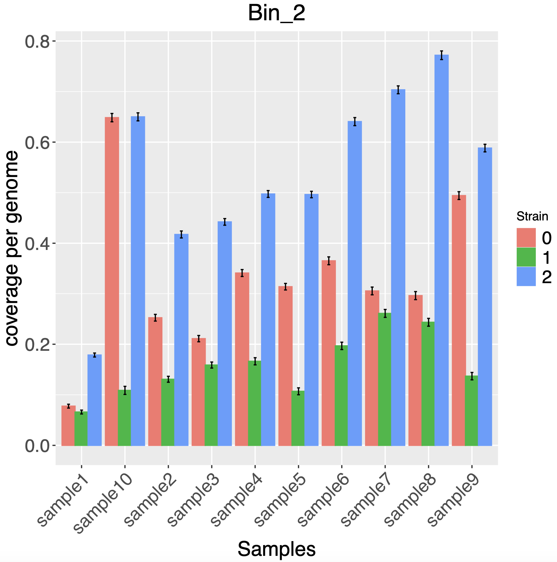
We can also look at the time series of strain abundances:

cp ~/repos/strain_resolution_practical/scripts/GammaPlot.R .
R
source('GammaPlot.R')
q()

Generate results

If the STRONG bayespaths step has finished we can generate results dir now:

cd /home/training/Projects/STRONG_AD
STRONG --config config.yaml STRONG_OUT results --threads 8 --verbose

The summary files gives information on number of mags, strains and taxonomy. Other files shows concatenation of Bin specific results.

Bin specific results

cd ~/Projects/STRONG_AD/STRONG_OUT/results/Bin_2

Joined graph is useful indicates that we have probably missed a strain on this example, this might be down to not running gene filtering or multiple NMF iterations.

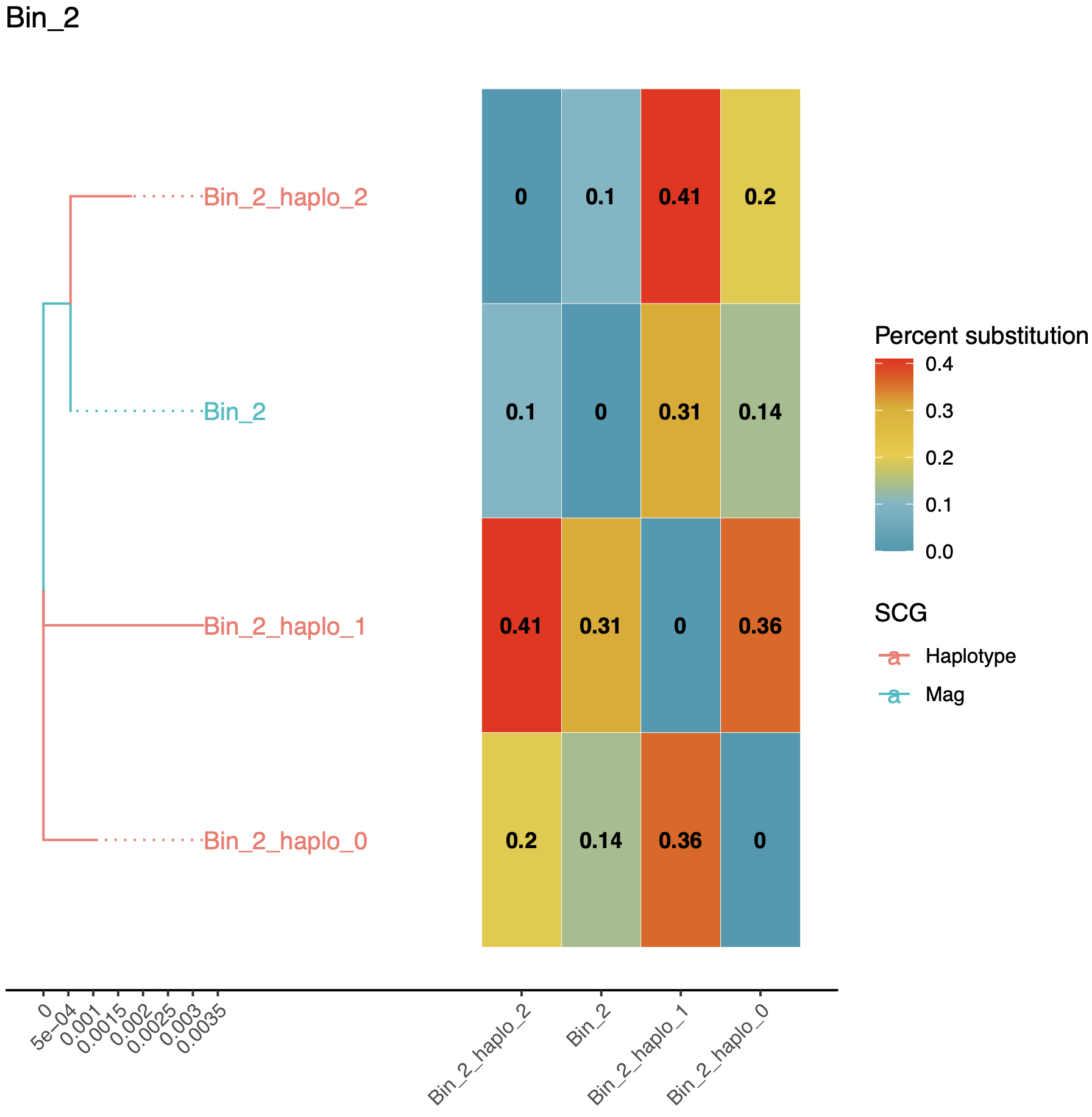
The haplotypes_tree.pdf has a phylogeny of strains and a heatmap giving percent divergences.

MAG taxonomy

STRONG will run gtdb on MAGs as standard but this is too slow and uses too much RAM. For now just have a look at the pre-run results:

cd ~/Projects/STRONG_AD/STRONG_OUT
ln -s ~/repos/strain_resolution_practical/STRONG_prerun/results result_prerun

Have a look at the summary file to find out the identity of the MAGs.

more summary.tsv

To run gtdb you need to add a line inside the config file with the path to gtdb database.

Extra things

Can you run STRONG with metabat2?

Can you taxonomically assign contigs with Kraken?