Multiple output Gaussian processes in MATLAB including the latent force model.
This page describes examples of how to use the Multi-output Gaussian Process Software (MULTIGP).
This software depends on the GPmat repository software.
Contains updates to the code for the technical report.
Updates to allow variational outputs for working with latent functions
that are white noise processes.
This is the very first version of the multi-ouput Gaussian Process toolbox. It shows toy examples for a full covariance model and two approximations proposed in the paper Sparse Convolved Gaussian Processes for Multi-ouput regression
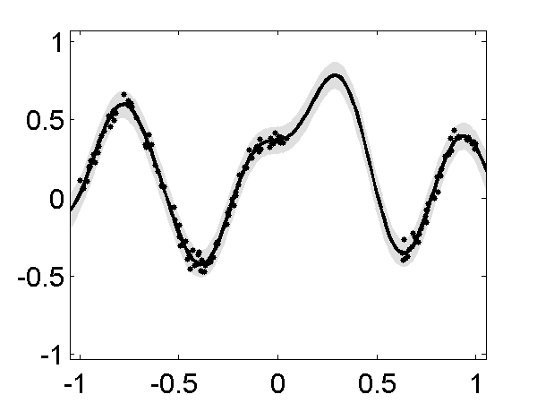
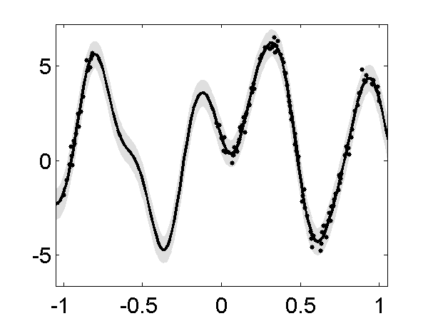
This example shows how it is possible to make multiple regression over four outputs using a Gaussian process constructed with the convolution process approach. Note that there are some ranges of missing data for outputs one and four.
>> demGpToy1Left First output in the four outputs of the demo. Right Fourth output for the same example.
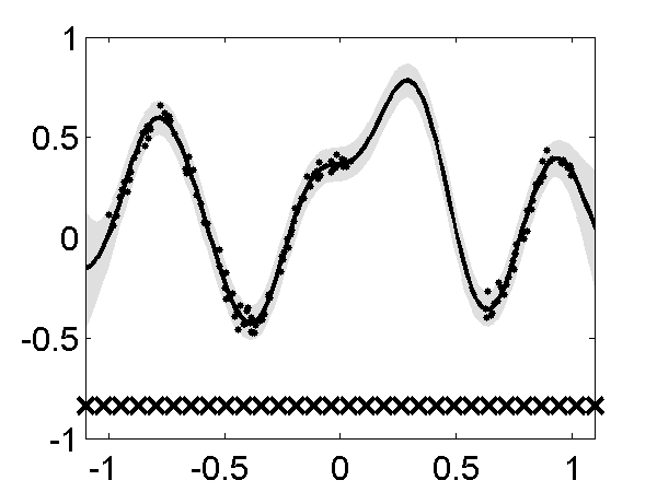
Multi-output Gaussian process using the PITC approximation and the FITC approximation (fixed inducing points)
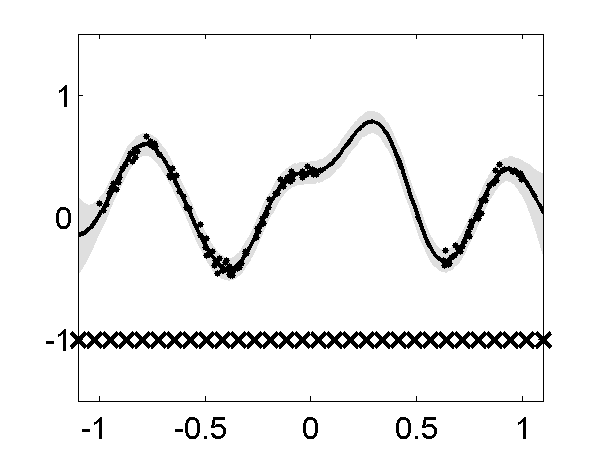
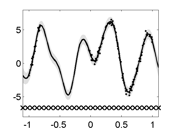
In the paper, two approximations that exploit conditional independencies in the model were proposed. Due to their similarities with the PITC and FITC approximations for the one output case, these multi-output approximations are named in a similar way. For PITC run
>> demSpmgpGgToy1For FITC run
>> demSpmgpGgToy2Up The same two outputs using PITC Down The same two outputs using FITC.
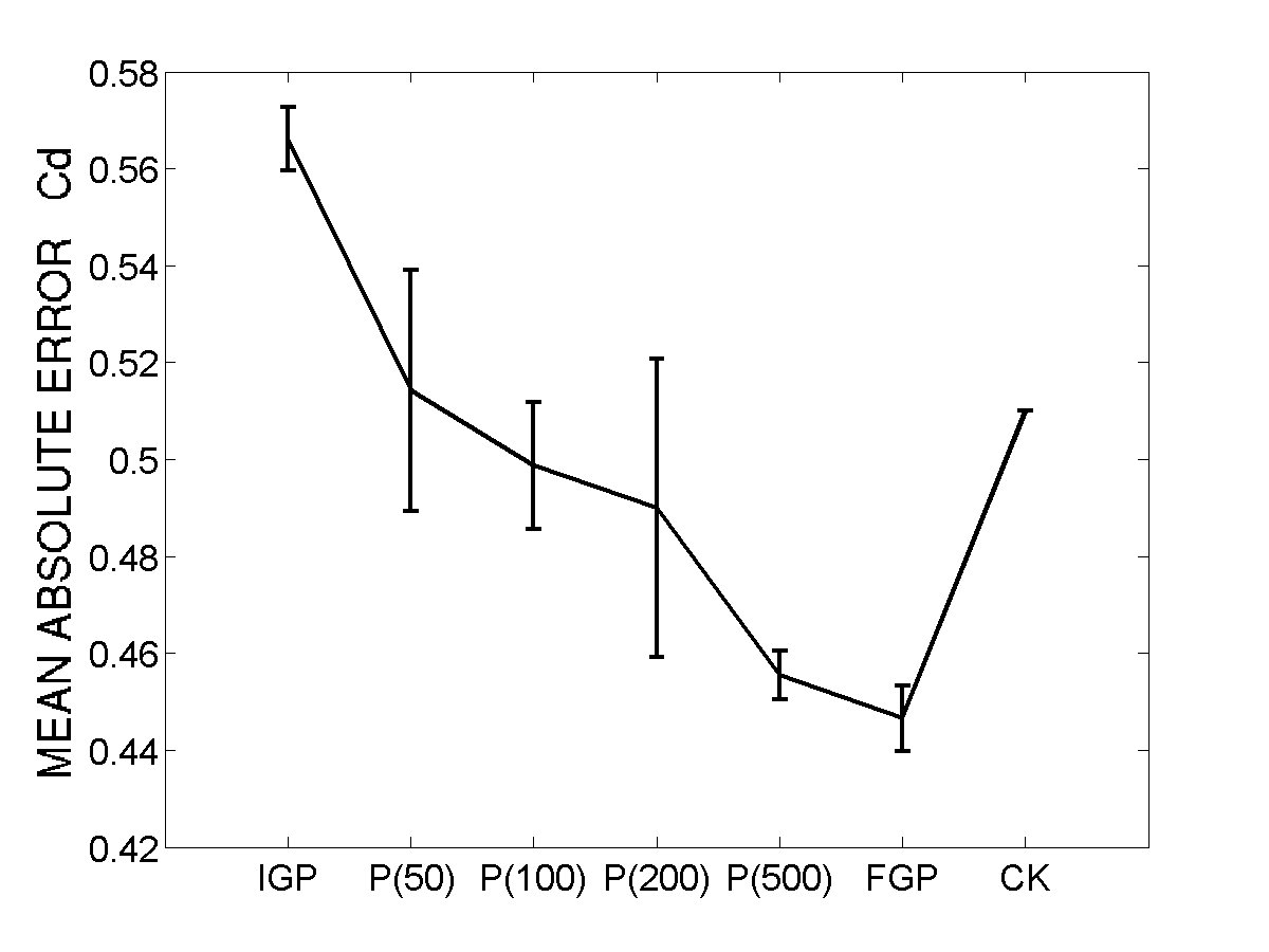
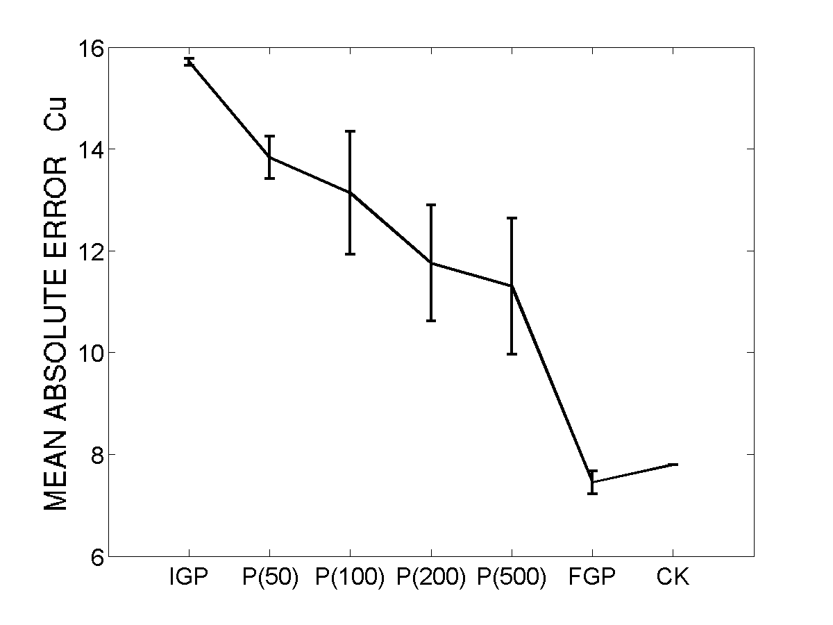
The experiment for the Swiss Jura Dataset using the full covariance matrix can be recreated using ( you will need to obtain the files prediction.dat and validation.dat from here. Go to the Publications link and then to the Book link)
>> demGgJuraThe result with the approximation can be recreated using
>> demSpmgpGgJuraMean absolute error and standard deviation for ten repetitions of the experiment for the Jura dataset In the bottom of each figure, IGP stands for independent GP, P(M) stands for PITC with M inducing values, FGP stands for full GP and CK stands for ordinary co-kriging. On the left, regression over Cadmium (Cd) and on the right, regression over Copper (Cu)
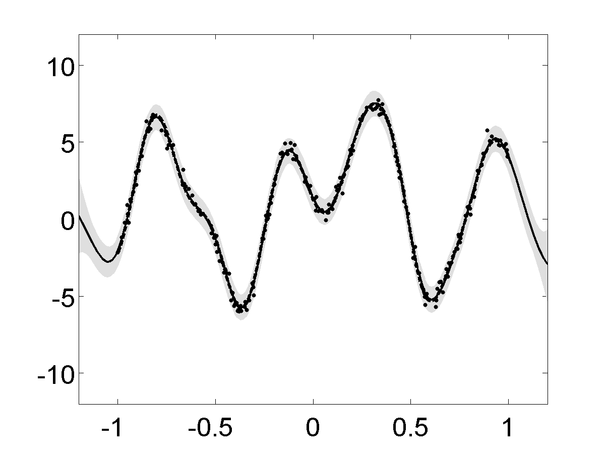
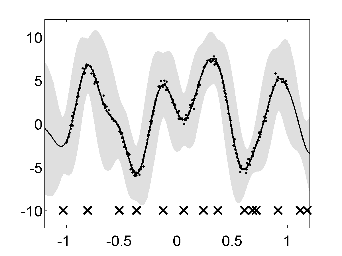
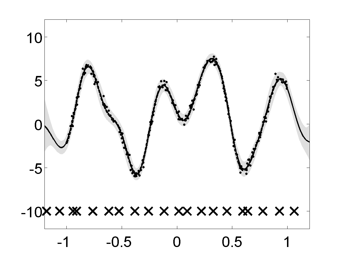
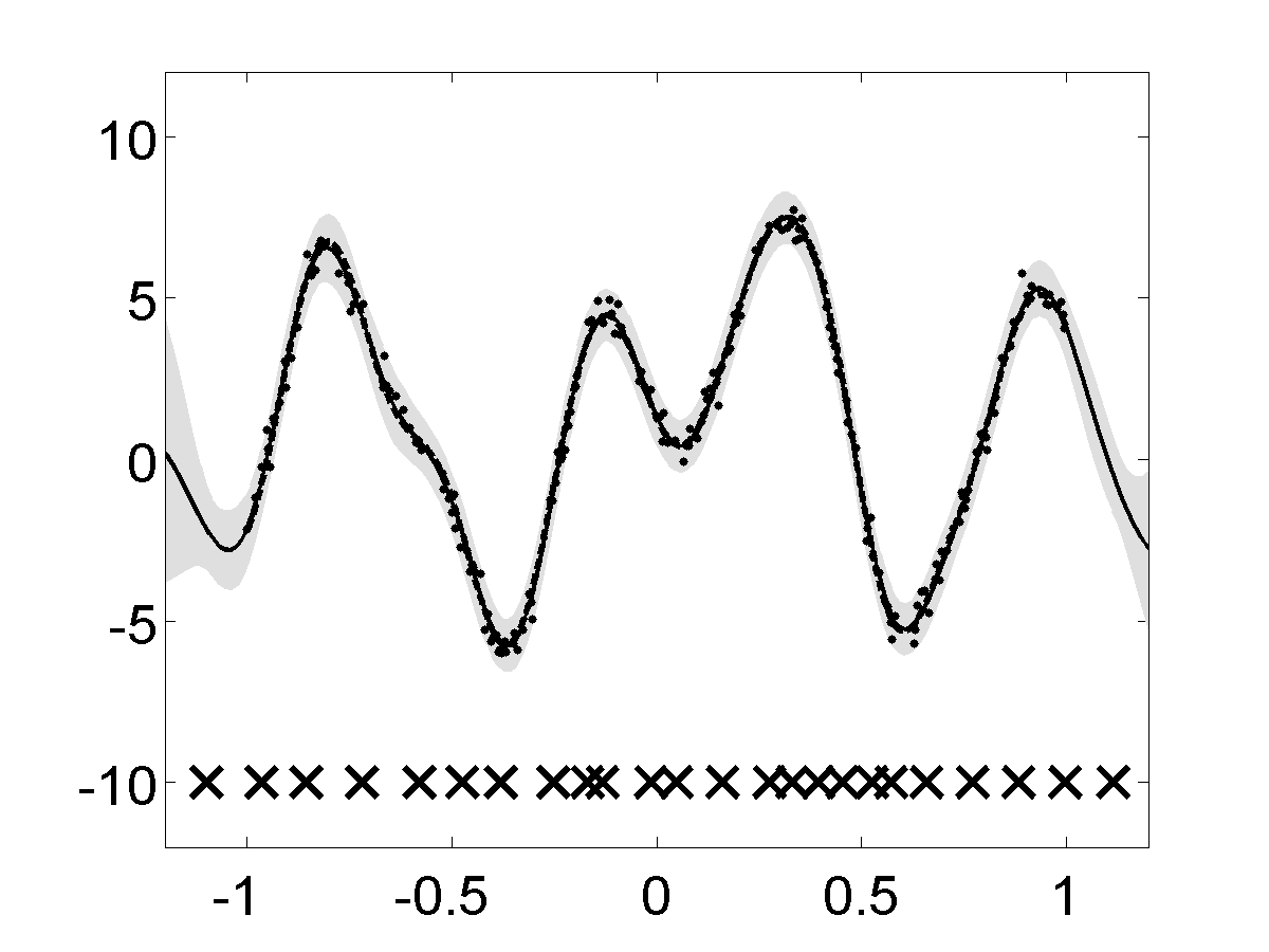
We generate a toy dataset consisting of four outputs, one latent function and one input dimension. The training data was sampled from the full GP. We generate 500 observation points for each output and use 200 observation points (per output) for training the full and the sparse multiple output GP. The figure 2 shows the training result. The predictions shown correspond to the full GP, the DTC approximation, the FITC approximation and the PITC approximation. For details of the setup refer to the paper. The difference with the previous toy example is that for this case we optimize the position of the inducing inputs.
To run the full GP, use
>> toy1DGgFTCExampleTo run the DTC approximation, use
>> toy1DGgDTCExample.mTo run the FITC approximation, use
>> toy1DGgFITCExample.mTo run the PITC approximation, use
>> toy1DGgPITCExample.mUp, Left Output four using full GP. Up, Right Output four using the DTC approximation. Output four using the FITC approximation. Down, Right Output four using the PITC approximation.
The goal is to predict the exam score obtained by a particular student belonging to a particular school. The data comes from the Inner London Education Authority (ILEA) (this dataset can be obtained here).
It consists of examination records from 139 secondary schools in years 1985, 1986 and 1987. It is a random 50% sample with 15362 students. From the multiple output point of view, each school represents one output and the exam score of each student a particular instantiation of that output. The results in terms of percentage of explained variance are shown in the figure.
To obtain the DTC approximation result, run
>> schoolGgDTCTo obtain the FITC approximation result, run
>> schoolGgFITCTo obtain the PITC approximation result, run
>> schoolGgPITC.m
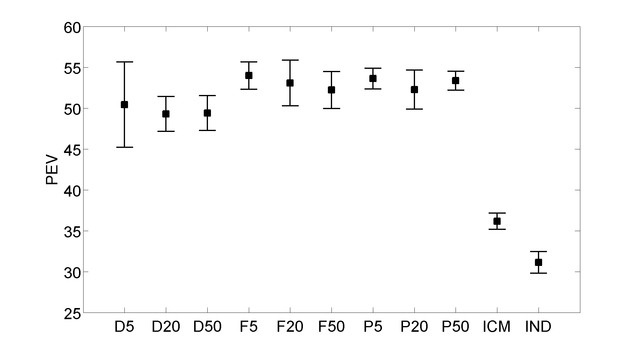
Mean and standard deviation of the percentage of explained variance for exam score prediction results on the ILEA dataset. The experiment was repeated ten times. In the bottom of the figure DK, FK, PK stands for DTC, FITC and PITC with K inducing values, respectively, ICM stands for intrinsic coregionalization model and IND stands for independent GPs. The ICM and the independent GPs results were obtained from Bonilla et al. (2008).
The dataset can be obtained here. It contains the expression level for 24 time points of 1935 genes. The connectivity matrix is also provided. We use the SIM kernel to infer the activity of the transcription factor ACE2 and the transcription factor SWI5. Figure shows the shape of the inferred transcriptions. The PITC approximation is employed with 15 inducing inputs.
To train the model that allows to infer the transcription factor proteins in the figure, run
>> demSpmgpSimYeastSpellmanPitc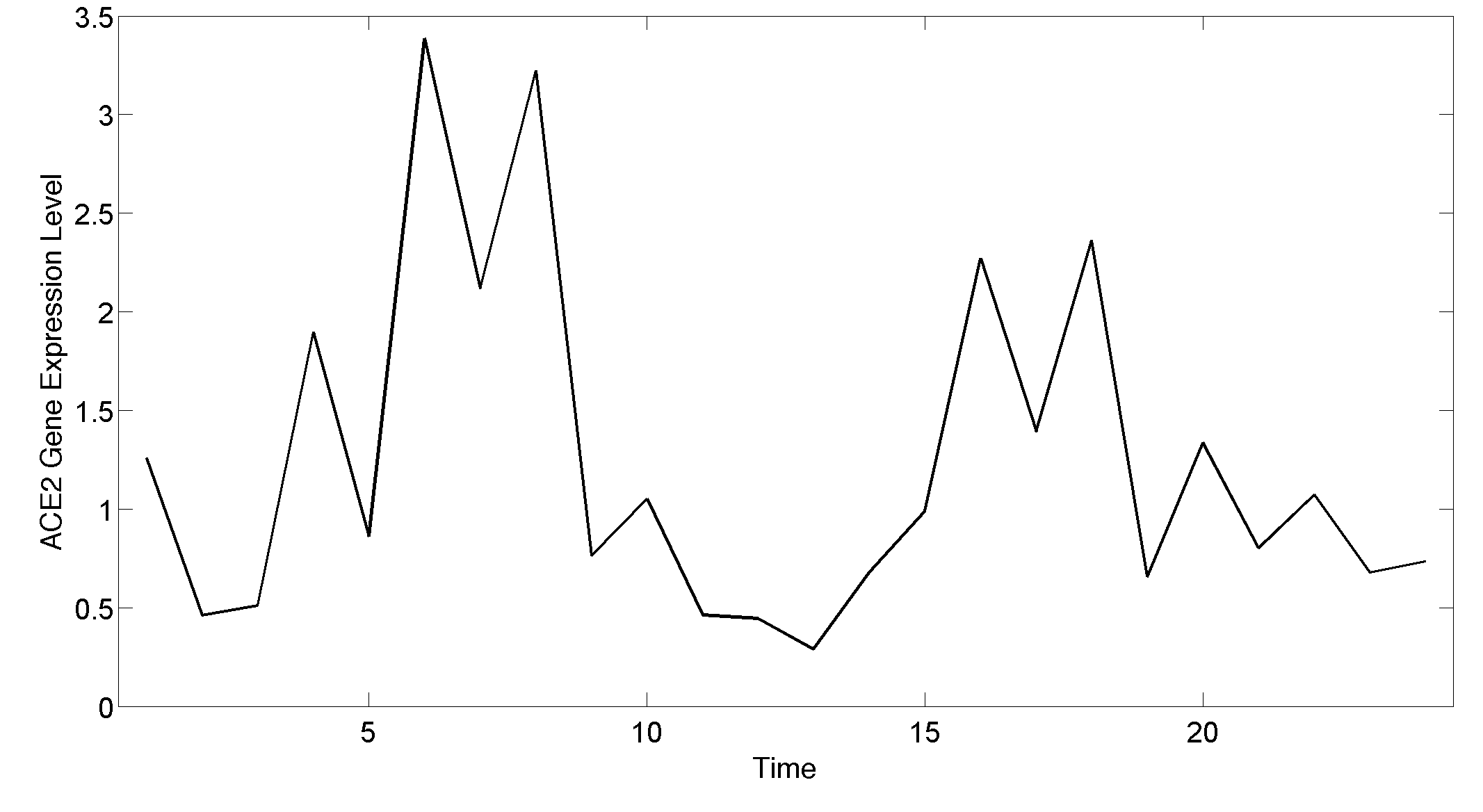
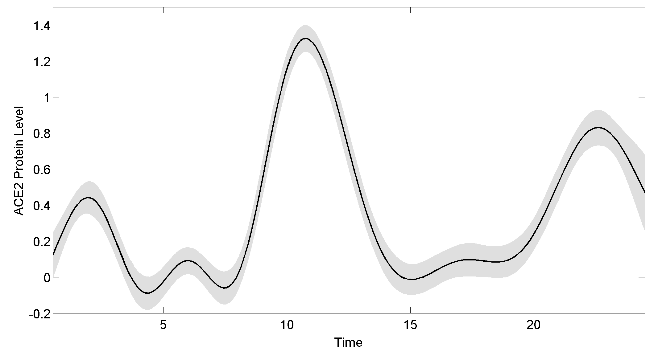
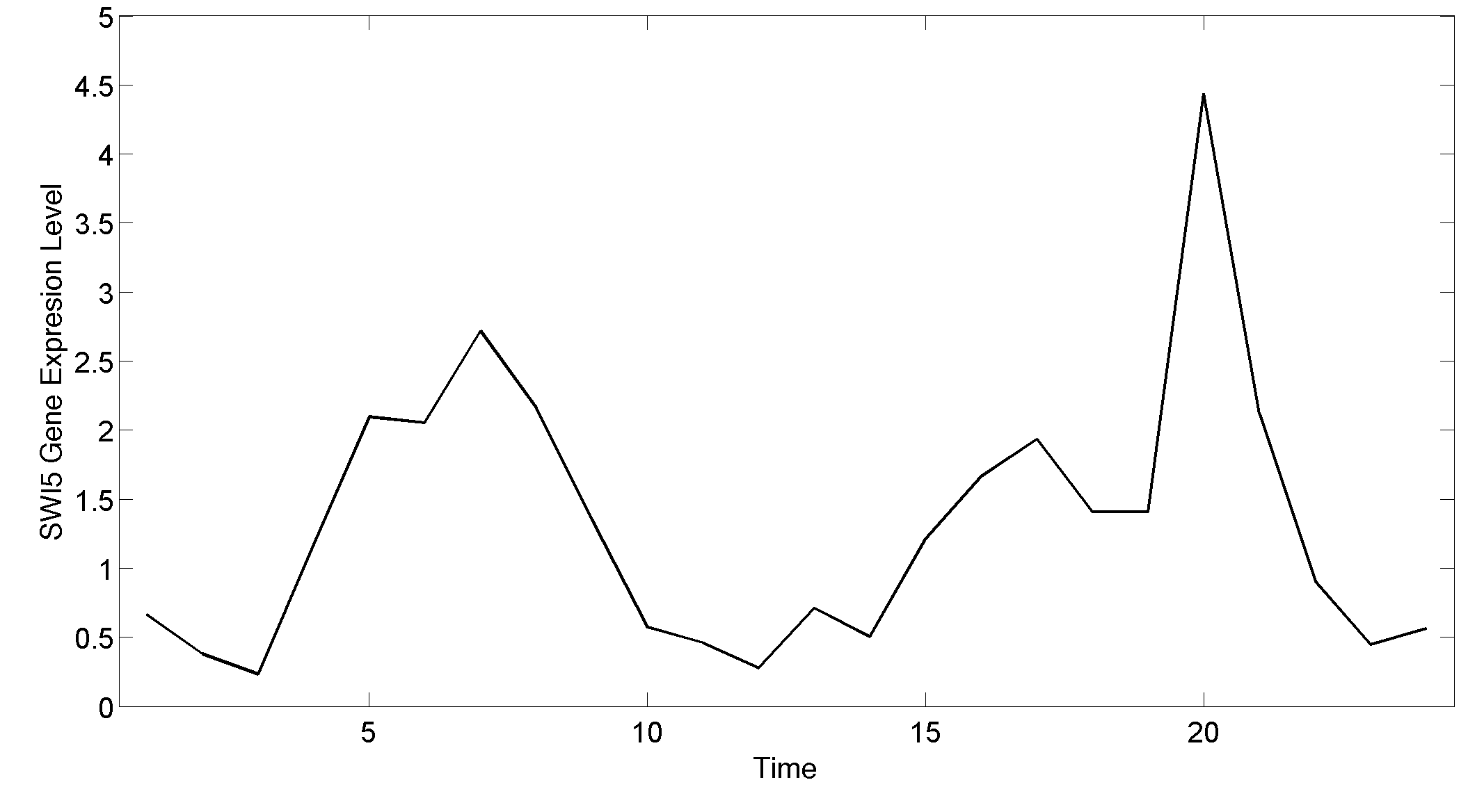
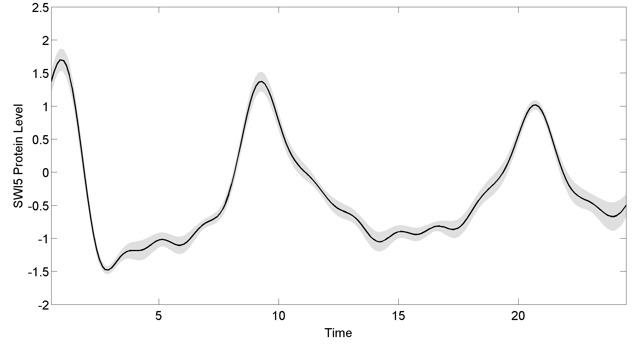
Gene expresion profile and inferred protein concentration for ACE2 and SWI5. The first column shows the gene expression level. The second column shows the mean posterior over the transcription factor and two standard deviations for the uncertainty. Up, Left Gene expression profile for ACE2. Up, Right Inferred protein concentration for ACE2. Down, Left Gene expression profile for SWI5. Down, Right Inferred protein concentration for SWI5.
