DySAT_main: A Python repository from Shi-D

DySAT: Deep Neural Representation Learning on Dynamic Graphs via Self-Attention Networks.

Contributors: Aravind Sankar (asankar3@illinois.edu).

Aravind Sankar, Yanhong Wu, Liang Gou, Wei Zhang, and Hao Yang, "DySAT: Deep Neural Representation Learning on Dynamic Graphs via Self-Attention Networks", International Conference on Web Search and Data Mining, WSDM 2020, Houston, TX, February 3-7, 2020.

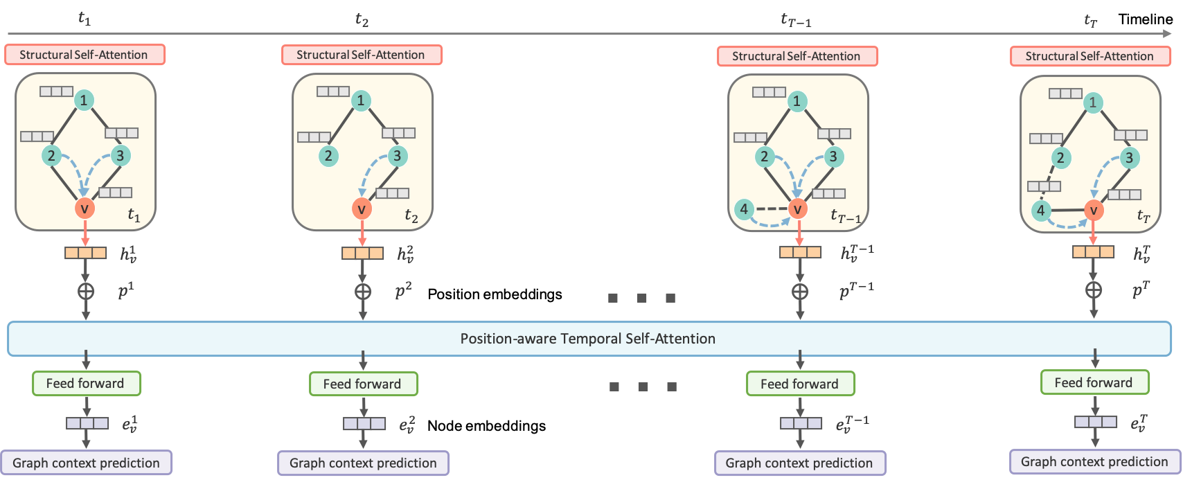
This repository contains a TensorFlow implementation of DySAT - Dynamic Self Attention (DySAT) networks for dynamic graph representation Learning. DySAT is an unsupervised graph embedding model to learn node embeddings in dynamic time-evolving attributed graphs, which may later be used for downstream application tasks such as link prediction, clustering and node classification.

Note: Though DySAT is designed for attributed dynamic graphs, our benchmarking experiments are carried out on datasets that do not have node attributes.

Incremental Dynamic Graph Embedding

To support streaming graph applications, we also provide an implementation of Incremental Self-Attention (IncSAT) Networks to learn dynamic incremental node embeddings in a stage-wise fashion. See our extended arxiv version for details on the algorithm.

If you make use of this code or the DySAT algorithm in your work, please cite our papers:

@article{sankar2018dynamic,
  title={Dynamic Graph Representation Learning via Self-Attention Networks},
  author={Sankar, Aravind and Wu, Yanhong and Gou, Liang and Zhang, Wei and Yang, Hao},
  journal={arXiv preprint arXiv:1812.09430},
  year={2018}
}

@inproceedings{sankar2020dysat,
  title={DySAT: Deep Neural Representation Learning on Dynamic Graphs via Self-Attention Networks},
  author={Sankar, Aravind and Wu, Yanhong and Gou, Liang and Zhang, Wei and Yang, Hao},
  booktitle={Proceedings of the 13th International Conference on Web Search and Data Mining},
  pages={519--527},
  year={2020}
}

Requirements:

Recent versions of TensorFlow (<= 1.14), numpy, scipy, sklearn, and networkx (<= 1.11) are required. The code has been tested under Python 2.7. The required packages can be installed using the following command:

$ pip install -r requirements.txt

To guarantee that you have the right package versions, you can use Anaconda to set up a virtual environment and install the dependencies from requirements.txt.

Input Format

In order to use your own data, you have to provide:

graphs: list of networkx graphs (or multigraphs) for each time step, saved as .npz files. Have a look at the load_graphs() and load_feats() functions in utils/preprocess.py for an example.
features: list of N x D feature matrices (N is the number of nodes and D is the number of features per node) in scipy sparse format) -- optional.

Repository Organization

data/ contains the necessary input file(s) for each dataset after pre-processing.
raw_data/ contains data pre-processing jupyter notebooks for reference.
models/ contains the implementation of two models - DySAT and IncSAT.
utils/ contains:
- preprocessing subroutines (preprocess.py, utilities.py, random_walk.py);
- minibatch iterators (minibatch.py, incremental_minibatch.py);
eval/ contains evaluation scripts that use simple logistic regression classifiers for link prediction based on the learnt node embeddings.

The pre-processed versions of all datasets are available here.

Running the code

The code can be run by executing python run_script.py. The default values of all parameters are set in the script file and can be specified as command line arguments. The most important arguments are min_time and max_time that specify the range of time steps to train the model. This script calls multiple instances of train.py (or train_incremental.py) with time steps in this range (both ends included).

For example, if min_time is 2 and max_time is 3, two instances of the model are trained, where the first one trains on the G₁, while the second instance trains on G₁ and G₂. In case of link prediction, the evaluation is performed on the links in G₂ for the first instance, and the links of G₃ for the second.

The other hyper-parameters of the model are specified in run_script.py (along with detailed descriptions) and may need to be appropriately tuned for different datasets.

Logging Directory

For logging, the model flag should be provided to specify the variant/version of the experimented model (initially set to default), in addition to choosing base_model as DySAT or IncSAT.

A logging directory log_dir is then created at ./logs/<base_model>_<model>/, overwriting any existing files that might conflict.

The output of the model, log files and evaluation results (on link prediction) will be stored in subdirectories of log_dir, with date-wise logged files, along with the set of hyper-parameters and settings used in the experiment.

The learnt embeddings will be stored in numpy formatted files at subdirectory output/ and the results of downstream evaluation tasks will be stored in a subdirectory csv/, within log_dir.

Shi-D/DySAT_main