Kinematics is the most basic study of how mechanical systems behave. In mobile robotics, we need to understand the mechanical behavior of robots both in order to design appropriate mobile robots for tasks and to understand how to create control software for an instance of mobile robot hardware. In this task, you will derive the inverse kinematic model of a four-wheeled omnidirectional robot shown in Figure 1, design a position controller and test it on the provided virtual experiments. The task requires v-rep (for visualization) and Matlab (coding) tools.
 Omnidirectional robot
Given
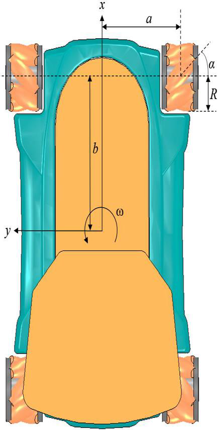
a=0.158516 m
b=0.228020 m
R=0.050369 45 m
α = 45˚
State : P=[𝑥 𝑦 𝜃 ]T
Omnidirectional robot
Given
a=0.158516 m
b=0.228020 m
R=0.050369 45 m
α = 45˚
State : P=[𝑥 𝑦 𝜃 ]T
-
The robot depicted in Figure 1 is a holonomic robot. Describe what it means for a robot to be holonomic. A mobile robot can use specially designed omniwheels or mecanum wheels to achieve omnidirectional motion, including spinning in place or translating in any direction are holonomic, meaning that they are configuration constraints. Four wheels design provides omni-directional movement for a robot without needing a conventional steering system and these robot ability system to move instantaneously in any direction from any configuration. These mechanism are called by holonomic constraint which have ability to travel in every direction under any orientation.
-
Derive the inverse kinematic model of this mobile robot
 Figure 2 Movement vector and coordinate system of given robot
Inverse kinematic model of the mobile robot is derived from the movement vector of four wheel drive mobile robot platform. Vector of the robot velocity v which has parallel direction to the x coordinate of Vx and Vy vector components are derived by
𝑉𝑥 = 𝑣 𝑐𝑜𝑠𝜃 𝑉𝑦 = 𝑣 𝑠𝑖𝑛 𝜃
𝜃 = lateral direction angle of robot movement velocity
𝜔 = Angular velocity of the robot at the center point of the mobile robot.
Linear velocity vector of the wheel and velocity of mecanum roller direction each wheel are indicated by Vi and RVi, respectively, where i is the corresponding wheel. Tilted angle, α between V and RV is 45° which represents the mecanum roller angle each wheels of αi: {π/4,- π/4,- π/4, π/4, }. Robot dimension is denoted by radius of a and b between body center robot and wheel axis of ai: {a, -a, -a, a} and bi: {b, b, -b, -b} where i : {1, 2, 3, 4} which represented wheel numbers. The velocity vector equation of the mobile robot toward coordinate system component can be calculated by
𝑉𝑖 + 𝑅∗𝑉𝑖 𝑐𝑜𝑠(α)= 𝑉𝑥 – ai∗𝜔 𝑅∗𝑉𝑖 𝑠𝑖𝑛(α)= 𝑉𝑦 + 𝑏𝑖∗𝜔
Using above 2 equation the linear velocity each wheel can be obtained:
𝑉𝑖=𝑉𝑥−𝑎𝑖∗ 𝜔−𝑉𝑦+𝑏𝑖∗𝜔tan (α 𝑖)
Since tan(𝑎i) are denotated above by tan(𝑎𝑖): {1, -1, -1, 1}, the
linear velocity of the mecanum wheel are:
𝑉1 = 𝑉𝑥 − 𝑉𝑦 − 𝑎𝜔 –𝑏𝜔 ……….(1)
𝑉2 = −𝑉𝑥 + 𝑉𝑦 + 𝑎𝜔 + 𝑏𝜔………(2)
𝑉3 = 𝑉𝑥 + 𝑉𝑦 − 𝑎𝜔 –𝑏𝜔…………..(3)
V4 = −Vx+ Vy + a𝜔 + b𝜔………..(4)
While the angular wheel velocities are Vi= 𝜔 *R and R is the radius of four mecanum wheels, Eq. (1)-(4) can be modified as:
Inverse Kinematics = [11−(𝑎+𝑏)−11(𝑎+𝑏)11−(𝑎+𝑏)−11(𝑎+𝑏)]1𝑅[𝑉𝑥𝑉𝑦𝜔]
The above equation shows mathematical model of the inverse kinematic
to be implemented to obtain angular velocities of each mecanum wheels by input of vector component of Vx, Vy and 𝜔 according to the lateral direction angle 𝜃 without changes the robot facing in certain direction.
Figure 2 Movement vector and coordinate system of given robot
Inverse kinematic model of the mobile robot is derived from the movement vector of four wheel drive mobile robot platform. Vector of the robot velocity v which has parallel direction to the x coordinate of Vx and Vy vector components are derived by
𝑉𝑥 = 𝑣 𝑐𝑜𝑠𝜃 𝑉𝑦 = 𝑣 𝑠𝑖𝑛 𝜃
𝜃 = lateral direction angle of robot movement velocity
𝜔 = Angular velocity of the robot at the center point of the mobile robot.
Linear velocity vector of the wheel and velocity of mecanum roller direction each wheel are indicated by Vi and RVi, respectively, where i is the corresponding wheel. Tilted angle, α between V and RV is 45° which represents the mecanum roller angle each wheels of αi: {π/4,- π/4,- π/4, π/4, }. Robot dimension is denoted by radius of a and b between body center robot and wheel axis of ai: {a, -a, -a, a} and bi: {b, b, -b, -b} where i : {1, 2, 3, 4} which represented wheel numbers. The velocity vector equation of the mobile robot toward coordinate system component can be calculated by
𝑉𝑖 + 𝑅∗𝑉𝑖 𝑐𝑜𝑠(α)= 𝑉𝑥 – ai∗𝜔 𝑅∗𝑉𝑖 𝑠𝑖𝑛(α)= 𝑉𝑦 + 𝑏𝑖∗𝜔
Using above 2 equation the linear velocity each wheel can be obtained:
𝑉𝑖=𝑉𝑥−𝑎𝑖∗ 𝜔−𝑉𝑦+𝑏𝑖∗𝜔tan (α 𝑖)
Since tan(𝑎i) are denotated above by tan(𝑎𝑖): {1, -1, -1, 1}, the
linear velocity of the mecanum wheel are:
𝑉1 = 𝑉𝑥 − 𝑉𝑦 − 𝑎𝜔 –𝑏𝜔 ……….(1)
𝑉2 = −𝑉𝑥 + 𝑉𝑦 + 𝑎𝜔 + 𝑏𝜔………(2)
𝑉3 = 𝑉𝑥 + 𝑉𝑦 − 𝑎𝜔 –𝑏𝜔…………..(3)
V4 = −Vx+ Vy + a𝜔 + b𝜔………..(4)
While the angular wheel velocities are Vi= 𝜔 *R and R is the radius of four mecanum wheels, Eq. (1)-(4) can be modified as:
Inverse Kinematics = [11−(𝑎+𝑏)−11(𝑎+𝑏)11−(𝑎+𝑏)−11(𝑎+𝑏)]1𝑅[𝑉𝑥𝑉𝑦𝜔]
The above equation shows mathematical model of the inverse kinematic
to be implemented to obtain angular velocities of each mecanum wheels by input of vector component of Vx, Vy and 𝜔 according to the lateral direction angle 𝜃 without changes the robot facing in certain direction. -
Design a position and orientation controller for this mobile robot
Position and orientation controller is designed by using in-built discrete PID function in MATLAB. The PID uses Forward Euler transition method to control the system. C = pid(Kp,Ki,Kd,Tf,Ts) creates a discrete-time PID controller with sample time Ts. The controller is: 𝐶=𝐾𝑝+𝐾𝑖∗𝐼𝐹(𝑧)+𝐾𝑑∗𝑠𝑇𝑓+𝐷𝐹(𝑧) The PID used in our code is as below: ControllerX= pid(KPx, KIx, KDx,Ts); ControllerY= pid(KPy, KIy, KDy,Ts); ControllerH= pid(KPh, KIh, KDh,Ts); where, KPx, KIx, KDx , KPy, KIy, KDy, KPh, KIh, KDh are the gain values of Proportional ,integral and derivative in x,y directions and h angle. Ts is the sample time. The gain PID values and Ts value are chose appropriately to rectify the error and stabilese the robot. The feedback to the system is done by using feedback() function in MATLAB. sys = feedback(sys1,sys2) returns a model object sys for the negative feedback interconnection of model objects sys1,sys2. The destination is give using a matrix. The feedback function is used as follows in our code: 𝑝𝑜𝑠𝑖𝑡𝑖𝑜𝑛𝐸𝑟𝑟𝑜𝑟𝑥 = 𝑓𝑒𝑒𝑑𝑏𝑎𝑐𝑘 (𝐶𝑜𝑛𝑡𝑟𝑜𝑙𝑙𝑒𝑟𝑋,𝑑𝑒𝑠𝑡𝑖𝑛𝑎𝑡𝑖𝑜𝑛(1,1) − 𝑐𝑢𝑟𝑟𝑒𝑛𝑡𝑃𝑜𝑠𝑖𝑡𝑖𝑜𝑛(1,1)) 𝑝𝑜𝑠𝑖𝑡𝑖𝑜𝑛𝐸𝑟𝑟𝑜𝑟𝑦 = 𝑓𝑒𝑒𝑑𝑏𝑎𝑐𝑘 (𝐶𝑜𝑛𝑡𝑟𝑜𝑙𝑙𝑒𝑟𝑌,𝑑𝑒𝑠𝑡𝑖𝑛𝑎𝑡𝑖𝑜𝑛(1,2) − 𝑐𝑢𝑟𝑟𝑒𝑛𝑡𝑃𝑜𝑠𝑖𝑡𝑖𝑜𝑛(1,2));
- Integrate the mathematical model from Task(2) and controller from Task(3) into the provided Matlab script and run the simulations below. The simulation is based on the assumption that there is a sensor capable of measuring the absolute position of the robot and that the robot is initially at pose in the world. P0(0,0,0) .
a. Command the robot to move to pose in the world P1(1,0,0) .
b. Reset and command the robot to move to pose in the world P2(0,1,0)
c. Reset and command the robot to move to pose in the world P3(1,1,0)
d. Reset and command the robot to move sequentially from P0 P1 P2 P3 P0
e. During the execution of part (d), you will observe that your robot almost comes to a standstill before proceeding to a next waypoint. To avoid this, add more intermediate points between the given waypoints and a threshold to determine when to move the next waypoint without slowing down. This should result in a smoother path. You may hold the heading constant during the simulation.

Timing graph for Task 4d/e during simulation
 X-Y Co ordinate graph during simulation
Add more intermediate points using for loop as given in the supporting file.
The corresponding timing and X-Y co-ordinate graph is obtained .
X-Y Co ordinate graph during simulation
Add more intermediate points using for loop as given in the supporting file.
The corresponding timing and X-Y co-ordinate graph is obtained .
f. Given the world in Figure 2, extract key points and manually generate a path for your robot to solve the maze. The path should take into account the vehicle constraints to avoid collision. On completing the maze, your robot should celebrate by spinning clockwise twice followed by two counter-clockwise spins. The goal is marked by the red circle. For distance approximations, all gray blocks are 50cm* 10cm .
 The intermediate points of the path is generated and the code for the maze is written as in the file.
The corresponding timing and X-Y co-ordinate graph is obtained .
The intermediate points of the path is generated and the code for the maze is written as in the file.
The corresponding timing and X-Y co-ordinate graph is obtained .
 Timing graph for Task 4f during simulation
 X-Y Co ordinate graph during simulation
g. Lastly, design a control motion plan to drive your robot twice around the circular world depicted in Figure 5. The robot should drive twice in clock direction and twice in counterclockwise direction. The direction switching should happen automatically up on completion of the first two rounds. The heading should always be tangential to the circular obstacle.
 Circular path. Diameter of the obstacle is 3.6 m. Robot position is x=2.1m and y = 0m.
The MATLAB code to ensure the robot remains in a circular path is coded and implemented with all the necessary constraints. The robot is controlled with respect to X,Y axis and rotation about Z-axis.
The corresponding timing and X-Y co-ordinate graph is obtained .
The given supporting code rotates until 90degree and faces some issue, we are looking into it.
Circular path. Diameter of the obstacle is 3.6 m. Robot position is x=2.1m and y = 0m.
The MATLAB code to ensure the robot remains in a circular path is coded and implemented with all the necessary constraints. The robot is controlled with respect to X,Y axis and rotation about Z-axis.
The corresponding timing and X-Y co-ordinate graph is obtained .
The given supporting code rotates until 90degree and faces some issue, we are looking into it.
 Timing graph for Task 4g during simulation
 X-Y Co ordinate graph during simulation