Fault diagnosis.

Introduction
Features
Requirements
Installation
Usage
Project Structure
Data
Evaluation
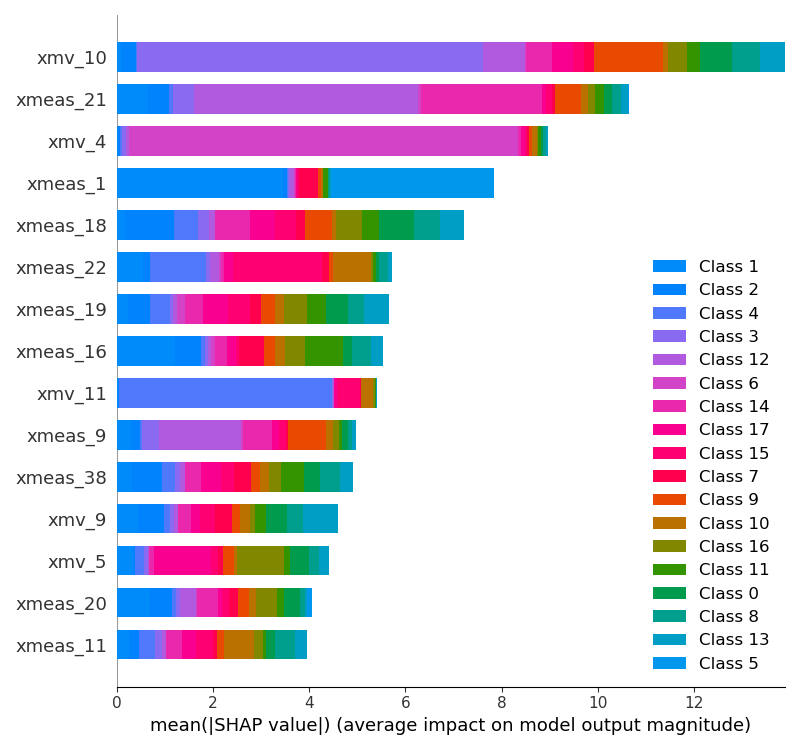
Explainable AI
Timeline
License
Credits

Introduction

Fault diagnosis is the process of diagnosis of fault in the machine after a failure occurs. To analyze the type of fault we use fault diagnosis. Here we used the Tennessee Eastman dataset. The Tennessee Eastman Process is a well-known benchmark process used to evaluate process control and fault detection methods. The goal of fault detection is to identify when the process is operating abnormally, which can lead to product quality issues, equipment damage, and safety hazards.

In this project, I trained ML models as mentioned below as well as a neural network model trained on Kggle GPU for the classification of the fault class type which has 52 features. I created a web dashboard which gives a glimpse of how prediction works If you are interested, you can try out. This predition also explains you which features are important for a particular feature with respect to model via explainable ai tools like Shap, Lime

For data analysis and model training refer

Requirements

Installation

# Example installation steps
git clone [https://github.com/ShreyashChacharkar/Fault-diagnosis](https://github.com/ShreyashChacharkar/Fault-diagnosis)
pip install -r requirements.txt

Usage

For data analysis and model training refer

For running web based app

python web-dashboard/app.py

Project Structure

Project's directories and files. Highlight the purpose of important files or folders.

project-root/
|-- dataset/
|   |-- raw/
|   |-- processed/
|-- notebooks/
|   |-- tep-fault-diagnosis-tree-classification.ipynb
|-- web-dashboard/
|   |-- static/
|       |-- style.css
|       |-- script.js
|   |-- templates/
|       |-- index.html 
|       |-- layout.html
|   |-- main.py
|   |-- utlis.py
|   |-- requirements.txt
|-- README.md
|-- requirements.txt

Data

Dataset link: kaggle source

This dataverse contains the data referenced in Rieth et al. (2017). Issues and Advances in Anomaly Detection Evaluation for Joint Human-Automated Systems. To be presented at Applied Human Factors and Ergonomics 2017.

Each .RData file is an external representation of an R dataframe that can be read into an R environment with the 'load' function. The variables loaded are named ‘fault_free_training’, ‘fault_free_testing’, ‘faulty_testing’, and ‘faulty_training’, corresponding to the RData files.

Each dataframe contains 55 columns:

Column 1 ('faultNumber') ranges from 1 to 20 in the “Faulty” datasets and represents the fault type in the TEP. The “FaultFree” datasets only contain fault 0 (i.e. normal operating conditions).
Column 2 ('simulationRun') ranges from 1 to 500 and represents a different random number generator state from which a full TEP dataset was generated (Note: the actual seeds used to generate training and testing datasets were non-overlapping).
Column 3 ('sample') ranges either from 1 to 500 (“Training” datasets) or 1 to 960 (“Testing” datasets). The TEP variables (columns 4 to 55) were sampled every 3 minutes for a total duration of 25 hours and 48 hours respectively. Note that the faults were introduced 1 and 8 hours into the Faulty Training and Faulty Testing datasets, respectively.
Columns 4 to 55 contain the process variables; the column names retain the original variable names.

for data preprocessing refer:

TEP data analysis

#.rdata file reader
import pyreadr

#zipfile extract
import zipfile as zp

#extract from zipfile
with zp.ZipFile("dataset\TEP_FaultFree_Training.RData (1).zip", 'r') as zip_ref:
    zip_ref.extractall("dataset")

# pyreadr converts rData into dictionary type object.
result = pyreadr.read_r("dataset/TEP_Faulty_Training.RData")
result1 = pyreadr.read_r("dataset/TEP_FaultFree_Training.RData")

#dataframes
df_train = result['faulty_training']
df_ff = result1['fault_free_training']


#save in csv file
df_ff.to_csv("dataset/fault_free_training.csv")
df_train.to_csv("dataset/faulty_training.csv")

Evaluation

Method	Accuracy
XG Boost	0.924
Random Forest	0.895
Naive Bayes	0.652
KNN	0.464
Decision Tree	0.827
Logistic Regression	0.695
Neural Networks	0.946

Explainable AI

Lime
Permutation importance
Partial dependence
Shap (local)
Shap (global)

eg.

Timeline

Days	Tasks	Description
Day 1	Topic introduction	read research paper, youtube, article
Day 1 to 2	Data wrangling	Data preprocessing (pyredr lib.), Cleaning, ETL activities, Data analysis, Data visualisation(matplotlib, seaborn)
Day 3	Model Training	Training with data(sklearn, TensorFlow, classification algorithm), Feature extracting, Hyperparameter Tuning
Day 4	Communication Result	Explainable AI Shaply and Lime, Real-time fault analysis
Day 5 to 8	Web dashboard	Web dashboard (baseline with templates, style, app.py, utlis.py)
Day 9	Deploying on cloud	Deploying selected ML model on GCP and AWS connect apis

License

This GitHub repository can be used for educational purposes only

ShreyashChacharkar/Fault-diagnosis