A team of data analytics consultants, referred to as the "Red Team," was tasked to transform data into information that provided profit-maximizing business insight for video game sales. To accomplish the task, the team used Python to build and evaluate several Machine Learning (ML) models (e.g.,Logistic regression, Neural Network) to determine which one was best suited for the scenario. Using ML enabled the team to leverage existing algorithms to learn from the data and lead to more accurate predictions.
For this project, the team attempted to predict the binary outcomes of potential profits for a video game launch in the European region. The team decided to build a Logistic Regression model in order for it to analyze the available data and when presented with a new sample, mathematically determines its probability for belonging to a class.
Once the model was completed, its performance was evaluated to see how well it predicted the binary outcomes.
Predicting video game sales was considered to be an interesting and fun topic to analyze. Video games have been around for many years and have evolved significantly over time; it is a huge market that provides entertainment for children and adults alike. Game development is also becoming increasingly common in many organizations that want to be part of its growing revenue stream.
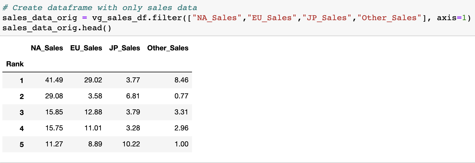
A CSV dataset, named vgsales.csv, was used for the analysis. The dataset contained 16,599 rows and the following columns:
- Rank: The ranking of overall sales
- Name: The name of the games
- Platform: The platform of the games release
- Year: The year the game was released
- Genre: The genre of the game
- Publisher: The publisher of the game
- Sales (NA, EU, JP, Other, Global): Sales in North America, Sales in Europe, Sales in Japan, Sales in the rest of the world, and Total worldwide sales
Will sales in Europe be greater than the target revenue?
The data was initially explored to determine which columns to keep as features and which columns to drop. The following are the columns dropped and retained for analysis.
- Dropped columns: Name, Year, Publisher, Other_Sales, Global Sales.
- Retained columns: Platform, Genre, NA_Sales, EU_Sales, JP_Sales
The columns Name and Publisher were dropped due to a large number of unique values, which were not very useful for the ML model. The Global_Sales column was dropped because it was a sum of the regional sales numbers. The team debated whether or not to keep Other_Sales column, but ultimately it was dropped. The Other_Sales column represented all sales outside of NA, EU, and JP, and the team felt that in a real-world application, this data would likely not be available prior to launching a video game in a major market. The data that was kept for analysis was reviewed for null values. Fortunately, no null values were found, so the team proceeded with the analysis.
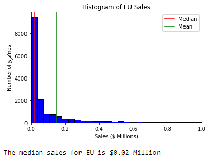
As stated above, the team strategically selected which columns to drop and keep to properly train the ML model. The string columns were encoded into numerical values. Scaling was explored with the sales data, but it was found that scaling did not improve the accuracy of the ML model. The team believed this could be due to the heavily skewed distribution of the sales data as indicated by the EU_Sales histogram below. Further investigation was required.
The target data was segregated from the feature data, and these two datasets were split into the training and testing sets using the train_test_split method built into scikit-learn as shown below.
The stratify parameter was set to y to maintain the same proportion of 0 and 1 values between the training and test sets. Note the class imbalance between 0 instances and 1 instances in our training data. This was handled with random oversampling as described below.
After lengthy consideration, the team elected to build a Logistic Regression model for this data. The Logistic Regression model was chosen because the question the team was trying to answer was a binary classification problem. The Logistic Regression model was advantageous in this case because it was easy to implement and easy to understand. Furthermore, the data included a limited number of features prior to categorical variable encoding, and the team was concerned that a complex model might overfit the data as a result.
One potential drawback to Logistic Regression model was related to the size of the data and the convergence of the model. Several optimizers were explored, and it was found that some optimizers required a significant number of iterations for the model to converge. Hyperparameter tuning was also investigated in an attempt to improve the model performance, but the team observed that there was not much to be gained in terms of model accuracy via hyperparameter tuning.
As mentioned previously, the training data, in its raw form, contained a fairly large class imbalance between 0 instances and 1 instances. In order to mitigate the class imbalance and optimize the model performance, random oversampling was used to balance the values in the 0 class and the 1 class as shown in the image below.
The image above also shows the training method used for the Logistic Regression model. The model was trained on the resampled training data using the lbfgs solver with a maximum of 200 iterations.
The accuracy score was approximately 88% as shown in the figure below. The precision for 0 and 1 instances are 0.93 and 0.74, respectively, and the recall for 0 and 1 instances 0.91 and 0.78, respectively.
This model addressed the question of whether or not sales in Europe will meet threshold sales by predicting a 1 or a 0 where a 1 indicates that European sales is expected to exceed the threshold, and a 0 indicates that European sales is not expected to exceed the threshold.
To investigate the model performance, the histograms below show the probability scores for 0 predictions and 1 predictions.
For 0 predictions, the probability histogram shows that most probabilities were above 0.75 to predict a 0.
For 1 predictions, the probability histogram shows a fairly even distribution of probabilities until the probability approaches 1 where a significant number of probabilities were at or near 1. This indicated that the model was very confident in its ability to predict 1 values, but the strong concentration of very high probabilities invites further investigation.
To gain further insight into the model performance, the image below shows the 0/1 predictions along with a line plot showing the corresponding probabilities. Note that this data supports the histograms above for the 0 and 1 predictions where the 0 portion of the probability curve shows a relatively flat slope from near 0 to roughly 0.25, and the 1 portion of the probability curve shows a rapid slope from 0.5 to nearly 1 where the curve flattens out.
ERD:
The team utilized Heroku for the online database. After cleaning the data and considering the constraints from Heroku regarding row limits, the data was divided into three categories: games, platforms, and genres. Once these categories were established, three CSV files were generated (using vg_db_csv_creator.ipynb) to populate the table data in pgAdmin and uploaded into the Heroku database.
CSV Data Imported into pgAdmin:
Data Uploaded into Heroku:
After the data was loaded into Heroku, a connection was established using heroku_db_connection.ipynb. Using SQL to query the online database, the team was able to perform two INNER JOINS to reconstruct the data needed for the ML and pass it into the Logistic Regression model for processing (DB_VG_LR_resample_Final.ipynb).
https://docs.google.com/presentation/d/1wRn_DMTICQlc5AWBJ5g96msv_DWjqQZWoBNYVVqalm4/edit?usp=sharing
https://docs.google.com/presentation/d/1xscv3WHg-kAVCQeLhKaqSvw58ImNI4yrhc5Y1BQruPc/edit?usp=sharing
-
https://www.kaggle.com/gregorut/videogamesales?select=vgsales.csv, accessed 2 July, 2021.
-
https://techcrunch.com/2015/10/31/the-history-of-gaming-an-evolving-community/, accessed 3 July, 2021.
-
https://github.com/get-icon/geticon/raw/master/icons/visual-studio-code.svg, accessed 15 July, 2021.
-
https://github.com/get-icon/geticon/raw/master/icons/python.svg, accessed 15 July, 2021.
-
https://github.com/get-icon/geticon/raw/master/icons/postgresql.svg, accessed 15 July, 2021.
-
https://maxgentechnologies.com/images/intern/python_machine_logo.jpg, accessed 15 July, 2021.
-
https://encrypted-tbn0.gstatic.com/images?q=tbn:ANd9GcSLPEwocsaSWuRA1_rvsYXMsXCMzgSWVB956N1CKMQ&usqp=CAU, accessed 15 July, 2021.
-
https://brand.heroku.com/static/media/heroku-logotype-spacing-vertical.dc54b577.svg, accessed 15 July, 2021.


