Coupled-VAE-Improved-Robustness-and-Accuracy-of-a-Variational-Autoencoder
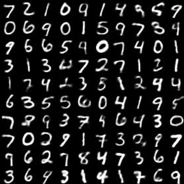
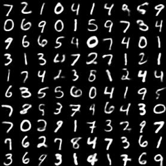
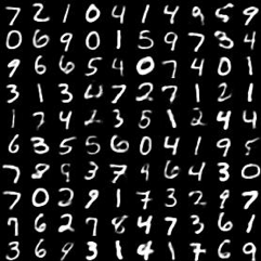
We present a coupled Variational Auto-Encoder (VAE) method that improves the accuracy and robustness of the probabilistic inferences on represented data. The new method models the dependency between input feature vectors (images) and weighs the outliers with a higher penalty by generalizing the original loss function to the coupled entropy function, using the principles of nonlinear statistical coupling. We evaluate the performance of the coupled VAE model using the MNIST dataset. Compared with the traditional VAE algorithm, the output images generated by the coupled VAE method are clearer and less blurry. The visualization of the input images embedded in 2D latent variable space provides a deeper insight into the structure of new model with coupled loss function: the latent variable has a smaller deviation and the output values are generated by a more compact latent space. We analyze the histograms of probabilities for the input images using the generalized mean metrics, in which increased geometric mean illustrates that the average likelihood of input data is improved. Increases in the -2/3 mean, which is sensitive to outliers, indicates improved robustness. The decisiveness, measured by the arithmetic mean of the likelihoods, is unchanged and -2/3 mean shows that the new model has better robustness.
Results
Output images with different k values
| Input image | k = 0 | k = 0.025 | k = 0.05 | k = 0.075 |
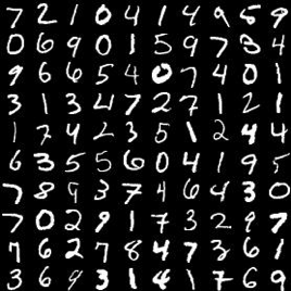
| 
| 
| 
| 
|
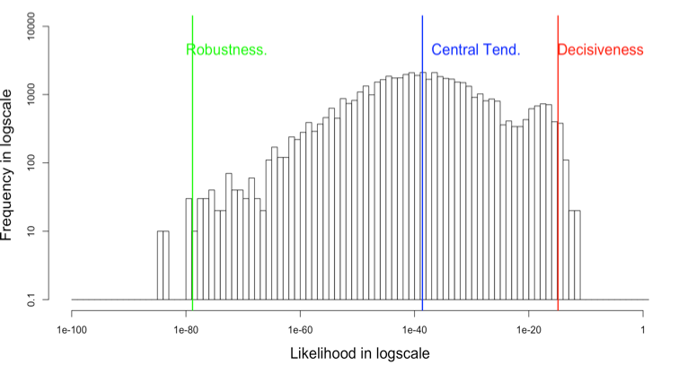
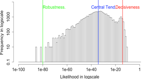
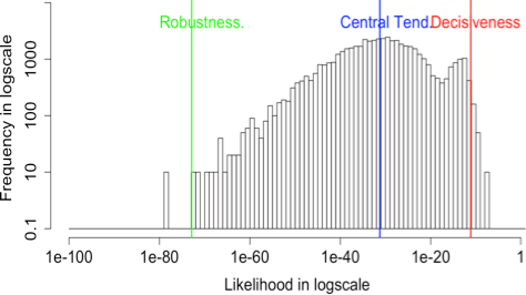
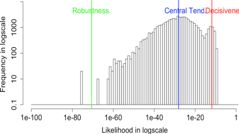
The histograms of likelihood for the input images with various k values
| k = 0 | k = 0.025 |
| 
|
| k = 0.05 | k = 0.1 |
| 
|
The relationship between coupling k with the probabilities for input data
| Coupling k | Arithmetic mean metric | Geometric mean metric | -2/3 mean metric |
|---|---|---|---|
| 0 | 1.31 × 10⁻¹⁵ | 2.4110 × -39 | 1.4010 × -79 |
| 0.025 | 6.6111 × -15 | 5.9810 × -35 | 9.9110 × -81 |
| 0.05 | 7.1810 × -12 | 5.8010 × -32 | 1.3110 × -73 |
| 0.1 | 1.3410 × -12 | 7.0910 × -29 | 2.5710 × -71 |
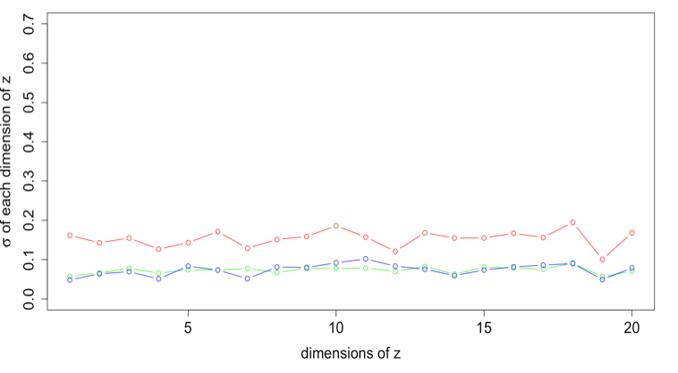
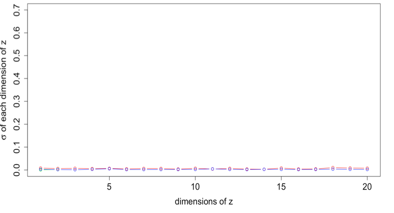
The standard deviation of latent variable samples near the three generalized mean metrics
| k = 0 | k = 0.025 |
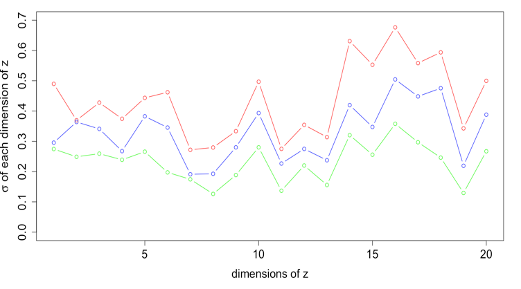
| 
|
| k = 0.05 | k = 0.1 |
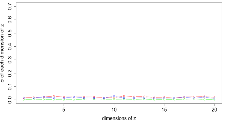
| 
|
The standard deviation of latent variable samples near the three generalized mean metrics (Magnified)
| k = 0.025 | k = 0.05 | k = 0.1 |
.png)
| .png)
| .png)
|
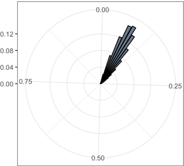
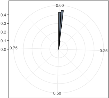
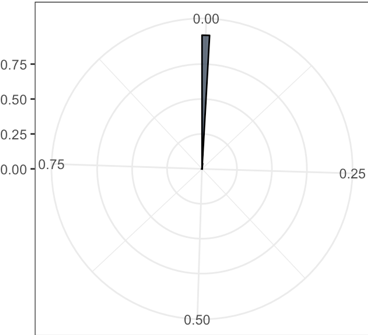
The rose plots of the various standard deviation values in 20 dimensions. The range of standard deviation reduces as coupling k increasing
| k = 0 | k = 0.025 | k = 0.05 | k = 0.1 |
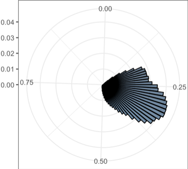
| 
| 
| 
|
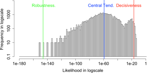
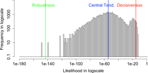
The histogram likelihood plots with a two-dimensional latent variable
| k = 0 | k = 0.025 |
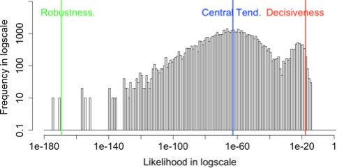
| 
|
| k = 0.05 | k = 0.075 |
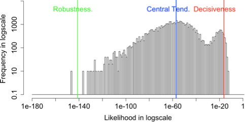
| 
|
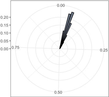
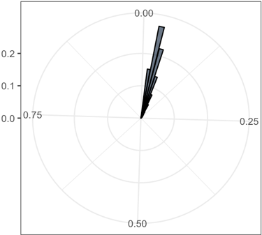
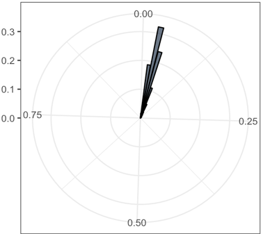
The rose plots of the various standard deviation values in 2 dimensions. The range of standard deviation reduces as coupling k increasing
| k = 0 | k = 0.025 | k = 0.05 | k = 0.075 |
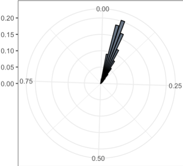
| 
| 
| 
|
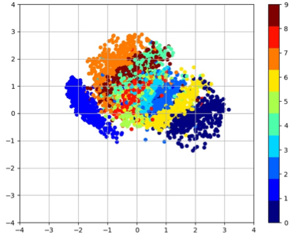
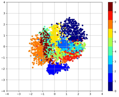
The plot of the latent space of VAE trained for 200 epochs on MNIST with various k values
| k = 0 | k = 0.025 | k = 0.05 | k = 0.075 |
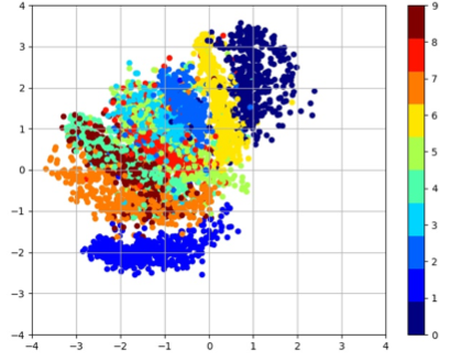
| 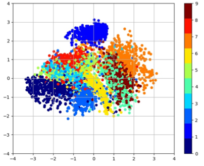
| 
| 
|
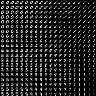
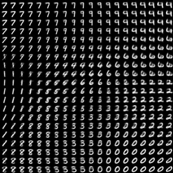
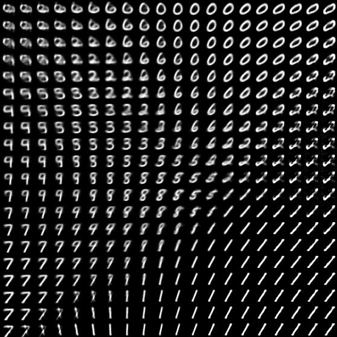
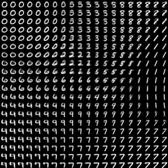
The plot of visualization of learned data manifold for generative models with the axes to be the values of each dimension of latent variables
| k = 0 | k = 0.025 | k = 0.05 | k = 0.075 |
| 
| 
| 
|
References
[1] D. P. Kingma and M. Welling, “Auto-Encoding Variational Bayes,” in International Conference on Learning Representations (ICLR), 2014, p. Arxiv: 1312.6114v10.pd.
[2] D. Tran, M. D. Hoffman, R. A. Saurous, E. Brevdo, K. Murphy, and D. M. Blei, “Deep probabilistic programming,” pp. 1–18, 2017.,
[3] S. R. Bowman, L. Vilnis, O. Vinyals, A. M. Dai, R. Jozefowicz, and S. Bengio, “Generating Sentences from a Continuous Space,” Nov. 2015.
[4] J. Zalger, “Application of variational autoencoders for aircraft turbomachinery design.”
[5] H. Xu et al., “Unsupervised Anomaly Detection via Variational Auto-Encoder for Seasonal KPIs in Web Applications,” in Proceedings of the 2018 World Wide Web Conference on World Wide Web - WWW ’18, 2018, pp. 187–196.
[6] K. P. Nelson and S. Umarov, “Nonlinear statistical coupling,” Phys. A Stat. Mech. its Appl., vol. 389, no. 11, pp. 2157–2163, Jun. 2010.
[7] K. P. Nelson, S. R. Umarov, and M. A. Kon, “On the average uncertainty for systems with nonlinear coupling,” Phys. A Stat. Mech. its Appl., vol. 468, pp. 30–43, Feb. 2017.
[8] K. P. Nelson, “Reduced Perplexity: A simplified perspective on assessing probabilistic forecasts,” Mar. 2016.
[9] C. Tsallis, Introduction to nonextensive statistical mechanics: approaching a complex world. 2009.
[10] O. Niemitalo, “A method for training artificial neural networks to generate missing data within a variable context,” 2010.
[11] T. Huang, Z. Zeng, C. Li, and C. Leung, “Neural Information Processing: 19th International Conference, ICONIP 2012, Doha, Qatar, November 12-15, 2012, Proceedings,” 2012.
[12] A. Rajaraman and J. D. Ullman, “Mining of massive datasets,” in Mining of Massive Datasets, 2011, vol. 9781107015, pp. 1–315.
[13] J. Donahue, P. Krähenbühl, and T. Darrell, “Adversarial Feature Learning,” May 2016.
[14] V. Dumoulin et al., “Adversarially Learned Inference,” Jun. 2016.
[15] J. Pearl, “Bayesian netwcrks: A model cf self-activated memory for evidential reasoning,” 1985.
[16] I. Goodfellow, Y. Bengio, and A. Courville, Deep learning. 2016.
[17] J. Ebbers, J. Heymann, L. Drude, T. Glarner, R. Haeb-Umbach, and B. Raj, “Hidden Markov Model Variational Autoencoder for Acoustic Unit Discovery,” 2017.
[18] N. Dilokthanakul et al., “Deep Unsupervised Clustering with Gaussian Mixture Variational Autoencoders,” Nov. 2016.,
[19] A. Srivastava and C. Sutton, “Autoencoding Variational Inference For Topic Models,” Mar. 2017.
[20] Yanna LeCun, Corinna Cortes, and Christopher J.C. Burges, “MNIST handwritten digit database, Yann LeCun, Corinna Cortes and Chris Burges.” [Online]. Available: http://yann.lecun.com/exdb/mnist/index.html. [Accessed: 18-Apr-2019].
[21] D. McAlister, “The law of the geometric mean,” Proc. R. Soc. London, vol. 29, no. 196–199, pp. 367–376, 1879.
[22] L. van der Maaten and G. Hinton, “Visualizing data using t-SNE,” J. Mach. Learn. Res., vol. 9, no. 2579–2605, p. 85, 2008.
Code References:
[1] https://github.com/tensorflow/tensorflow
[2] https://github.com/hwalsuklee/tensorflow-mnist-VAE
Acknowledgements
The results has been tested with Tensorflow r1.13.1 -Gpu-version on Windows 10.