SiyuanYan1/XDEnsembles

Robustness via Cross-Domain Ensembles

Robustness via Cross-Domain Ensembles [ICCV 2021, Oral]

This repository contains tools for training and evaluating:

• Pretrained models
• Demo code
• Training scripts
• Docker and installation instructions

for the paper: Robustness via Cross-Domain Ensembles.

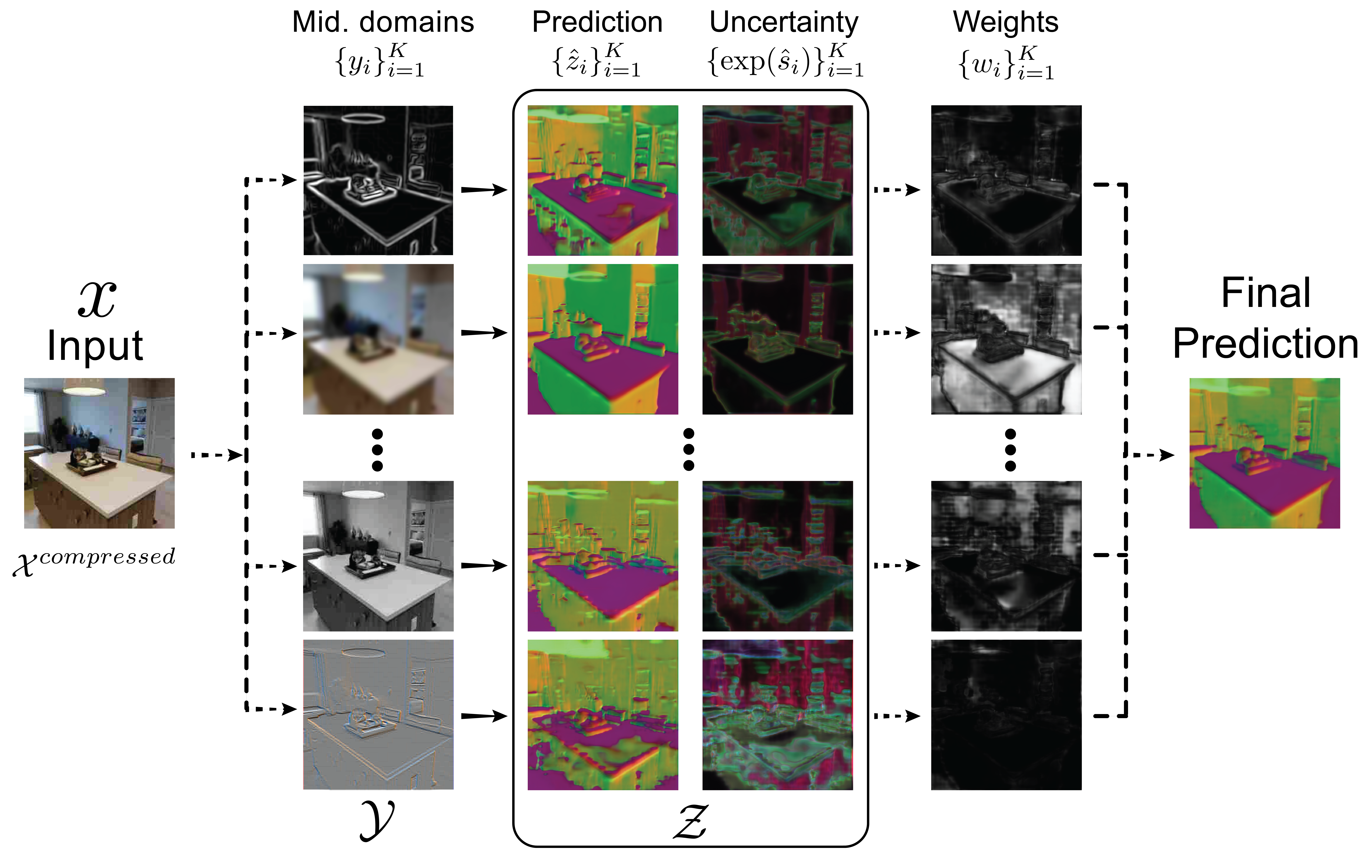
Above: An overview of the proposed method for creating a robust and diverse ensemble of predictions. A set of networks predict a target domain (surface normals) given an input image that has undergone an unknown distribution shift (JPEG compression degradation), via K middle domains (e.g. 2D texture edges, low-pass filtering, greyscale image, emboss filtering, etc). The prediction by each of the K paths are then merged into one final strong prediction using weights that are based on the uncertainty associated with each prediction. This method is shown to be significantly robust against adversarial and non-adversarial distribution shifts. In the figure above, solid and dashed arrows represent learned and analytical functions, respectively.

---

Table of Contents

• Introduction
• Installation
• Quickstart (demo code)
• Download all pretrained models
• Train a model
  • Instructions for training
  • To train on a new middle domain
  • To train on other datasets
  • CIFAR-100 classification (quickstart)
• Citing

Introduction

Robustness problem in neural networks: Neural networks deployed in the real-world will encounter data with naturally occurring distortions, e.g. motion blur, brightness changes, etc. Such changes make up shifts from the training data distribution. While neural networks are able to learn complex functions in-distribution, their predictions are deemed unreliable under such shifts, i.e. they are not robust. This presents a core challenge that needs to be solved for these models to be useful in the real-world.

Why do we need robust predictions? Suppose we want to learn a mapping from an input domain, e.g. RGB images, to a target domain, e.g. surface normals (see above figure). A common approach is to learn this mapping with a direct path, i.e. RGB → surface normals. Since this path directly operates on the input domain, it is prone to being affected by any slight alterations in the RGB image, e.g. brightness changes.

How do we obtain robust predictions? An alternative can be to go through a middle domain that is invariant to that change. For example, the surface normals predicted via the RGB → 2D edges → surface normals path will be resilient to brightness distortions in the input as the 2D edges domain abstracts that away. However, the distortions that a model may encounter are broad and unknown ahead of time, and some middle domains can be too lossy for certain downstream predictions. These issues can be mitigated by employing an ensemble of predictions made via a diverse set of middle domains and merging their (relatively weaker) predictions into one (stronger) output on-the-fly.

Middle and target domains

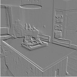
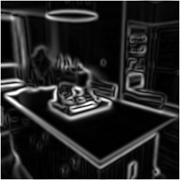
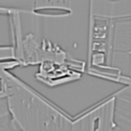
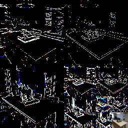
For the paper, we programmatically extracted the following middle domains from the RGB input (no learning, implementations are provided here):

Emboss         Greyscale               Sobel Edges            Laplace Edges         
Wavelet        Low-pass Filtered       Sharpened

A visualization of these middle domains for an RGB image can be seen below.

RGB	Emboss	Greyscale	Sobel Edges
Laplace Edges	Wavelet	Low-pass Filtered	Sharpened

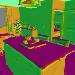
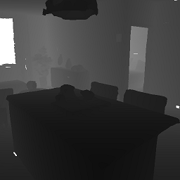
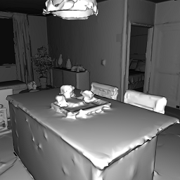
For target domains, we use the followings from the Taskonomy dataset:

Surface Normals          Depth (Z-Buffer)            Reshading

A visualization of target domains for an RGB image can be seen below.

RGB	Surface Normals	Depth (Z-Buffer)	Reshading

Quickstart

Download the trained networks

If you haven't yet, then download the pretrained models. Models used for the demo can be downloaded with the following command:

sh ./tools/download_models.sh

This downloads the single UNet baseline, deep ensembles, and cross-domain ensembles models for normal, reshading and depth_zbuffer targets (14GB) to a folder called ./models/. Individual models can be downloaded here.

Run a model on your own (clean) image

To run the trained model of a task on a specific image:

python demo.py --task $TASK --img_path $PATH_TO_IMAGE_OR_FOLDER --output_path $PATH_TO_SAVE_OUTPUT

The --task flag specifies the target task for the input image, which should be either normal, reshading or depth_zbuffer.

To run the script for a normal target on the example image:

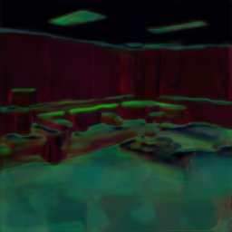
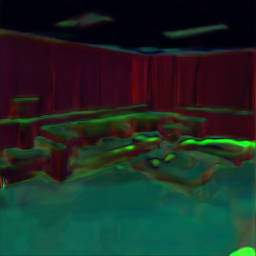
python demo.py --task normal --img_path assets/test.png --output_path assets/

It returns the output prediction (test_normal_ours_mean.png) and the associated uncertainty (test_normal_ours_sig.png) for the proposed method as well as the single UNet baseline and deep ensembles.

Distorted data

You can also apply distortion to your input from Common Corruptions to see how well the models handle the distribution shift.

python demo.py --task $TASK --img_path $PATH_TO_IMAGE_OR_FOLDER --output_path $PATH_TO_SAVE_OUTPUT --distortion $DISTORTION_NAME --severity $SEVERITY_LEVEL

• The argument --distortion can be set to one of the followings:

'shot_noise', 'speckle_noise', 'impulse_noise', 'defocus_blur', 'contrast', 'brightness','saturate', 'jpeg_compression', 'pixelate', 'spatter', 'glass_blur', 'gaussian_noise', 'gaussian_blur'

• The argument --severity can be set from 1 to 5 to change the severity of the applied distortion.

Example with pixelate distortion at severity 2:

python demo.py --task normal --img_path assets/test.png --output_path assets/ --distortion 'pixelate' --severity 2

Test image (distorted)		Baseline	Deep ensembles	Ours
	Prediction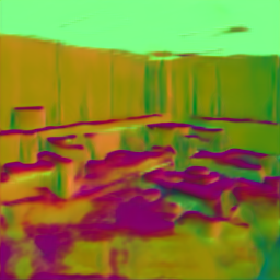
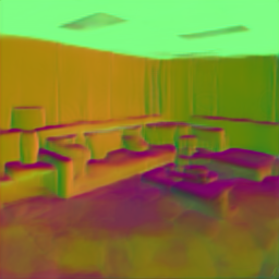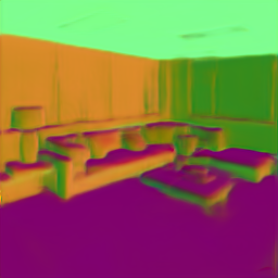	Uncertainty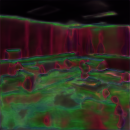

The distorted input is also saved as distorted_input.png in the output folder.

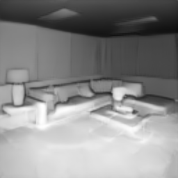
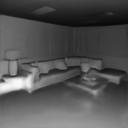
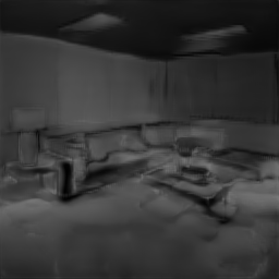
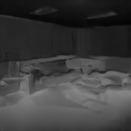
Similarly, running for target tasks reshading and depth gives the followings:

	Baseline (reshading)	Deep ensembles (reshading)	Ours (reshading)
Prediction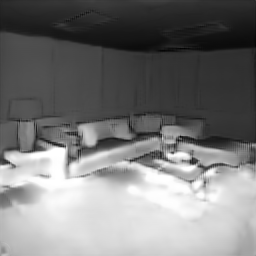
Uncertainty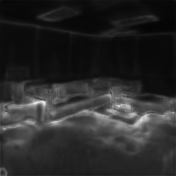

	Baseline (depth)	Deep ensembles (depth)	Ours (depth)
Prediction
Uncertainty

Pretrained models

Network Architecture

All networks are based on the UNet architecture. They take in an input size of 256x256, upsampling is done via bilinear interpolations instead of deconvolutions. All models were trained with an NLL loss. Architectural hyperparameters for the models are detailed in transfers.py.

Download the models

The following command downloads the final pretrained models.

sh ./tools/download_models.sh

This downloads the single UNet baseline, deep ensembles, and cross-domain ensembles models for normal, reshading and depth_zbuffer targets (14GB) to a folder called ./models/. Individual models can be downloaded here.

Download the models from different training stages

Our method includes three training stages: baseline training, consistency training (optional), and sigma training. The pretrained models for the first two stages can be downloaded here (9.3GB). These models were used for the ablation studies in the paper.

sh ./tools/download_baselines.sh

Download perceptual models

The pretrained perceptual models for the consistency training are the same as those used in Robust Learning Through Cross-Task Consistency. They can be downloaded with the following command.

sh ./tools/download_percep_models.sh

This downloads the perceptual models for the normal, reshading and depth_zbuffer targets (1.6GB). Each target has 7 pretrained models (from the other sources below).

Curvature         Edge-3D            Reshading
Depth-ZBuffer     Keypoint-2D        RGB       
Edge-2D           Keypoint-3D        Surface-Normal 

Perceptual model architectural hyperparameters are detailed in transfers.py, and some of the pretrained models were trained using L2 loss. For using these models with the provided training code, the pretrained models should be placed in the file path defined by MODELS_DIR in utils.py.

Individual perceptual models can be downloaded here.

Download other baselines

We also provide the models for other baselines used in the paper. The pretrained baselines can be downloaded here and the architectural details can be reached from transfers.py. Note that we will not be providing support for them.

• A full list of baselines is in the table below:

  Baseline Method	Description
  Baseline UNet [PDF]	UNets trained on the Taskonomy dataset.
  Baseline UNet + Adversarial training [PDF]	Baseline UNets (above) were finetuned with adversarial examples using I-FGSM (details can be reached from the paper).
  Multi-Task [PDF]	A multi-task model we trained using UNets, using a shared encoder (similar to here) to predict normal, reshading, and depth from the RGB input.
  Multi-Domain	Instead of a single input domain, we use all the middle domains and RGB as inputs, and output the prediction for a single task.

Installation

There are two convenient ways to run the code. Either using Docker (recommended) or using a Python-specific tool such as pip, conda, or virtualenv.

Installation via Docker [Recommended]

We provide a docker that contains the code and all the necessary libraries. It's simple to install and run.

1. Simply run:

docker run --runtime=nvidia -ti --rm ofkar/xdensembles:latest

The code is now available in the docker under your home directory (/XDEnsembles), and all the necessary libraries should already be installed in the docker.

Installation via Pip/Conda/Virtualenv

The code can also be run using a Python environment manager such as Conda. See requirements.txt for complete list of packages. We recommend doing a clean installation of requirements using virtualenv:

1. Clone the repo:

git clone https://github.com/EPFL-VILAB/XDEnsembles.git
cd XDEnsembles

2. Create a new environment and install the libraries:

conda create -n testenv -y python=3.6
source activate testenv
pip install -r tools/requirements.txt
apt-get update && apt-get -y install libmagickwand-dev && apt-get -y install libgl1-mesa-glx
git clone https://github.com/fbcotter/pytorch_wavelets && cd pytorch_wavelets && pip install .

Training

Assuming that you want to train on the full dataset or on your own dataset, read on.

Note that there are 3 stages of training: 1. baseline training, 2. consistency training (optional), and 3. sigma training. The pretrained models for the first two stages are provided here and the final models here.

Code structure

config/             # Configuration parameters: where to save results, etc.
    split.txt           # Train, val split
    jobinfo.txt         # Defines job name, base_dir
modules/            # Network definitions
train_baseline.py   # Script for baseline training 
train_cons.py       # Script for consistency training
train_sig.py        # Script for sigma training
train_merging.py    # Script for merging training
dataset.py          # Creates dataloader
energy_baseline.py  # Defines path config, computes total loss, plots for baseline training
energy_cons.py      # Defines path config, computes total loss, logging for consistency training
energy_sig.py       # Defines path config, computes total loss, logging for sigma training
energy_merging.py       # Defines path config, computes total loss, logging for merging training
models.py           # Implements forward backward pass
graph.py            # Computes path defined in energy.py
task_configs.py     # Defines task specific preprocessing, masks, loss fn
transfers.py        # Loads models
utils.py            # Defines file paths (described below), analytical operations to get middle domains
distortions.py      # Implemementations of common corruptions
demo.py             # Demo script

Expected folder structure

The code expects folders structured as follows. These can be modified by changing values in utils.py

base_dir/                   # The following paths are defined in utils.py (BASE_DIR)
    shared/                 # with the corresponding variable names in brackets
        models/             # Pretrained models (MODELS_DIR)
        results_[jobname]/  # Checkpoint of model being trained (RESULTS_DIR)
        ood_standard_set/   # OOD data for visualization (OOD_DIR)
    data_dir/               # taskonomy data (DATA_DIRS)

Steps

1. Train baseline models

• To train from RGB or one of the predefined middle domains, the command is given by

python train_baseline.py baseline_{input_domain}2{output_domain}

For example, to train a emboss to normal network, the command is

python train_baseline.py baseline_emboss2normal

This trains the model with negative log likelihood (NLL) loss. In addition to the prediction, the uncertainty is also predicted.

To train from new middle domain,

• Add its definition in utils.py. The expected input and output is of size 1xCxHxW.
• Add the model definition in the pretrained_transfers dictionary in transfers.py. A emboss transformation that has been added to utils.py as emboss_kernel will be added as

('rgb', 'emboss'):
   (lambda: emboss_kernel, None),

• In the energy_configs dictionary in energy.py, define the domains for the path. For rgb2emboss2normal,

    "baseline_emboss2normal": {
      "paths": {
          "x": [tasks.rgb],
          "y^": [tasks.normal],
          "n(x)": [tasks.rgb, tasks.emboss, tasks.normal],
      },
      ...
    }

The other required configs, "loss" and "plots", remain the same.

2. Sigma training

The above training step returns predicted uncertainties that are overconfident when given out of distribution data. In this step, train the uncertainties to generalize while holding the predictions fixed. The command is given by

python train_sig.py trainsig_{input_domain}{output_domain}

To train a emboss to normal network, the command is

python train_sig.py trainsig_embossnormal

3. Training with consistency (OPTIONAL)

Training with cross-task consistency constraints is optional. The command is given by,

python train_cons.py consistency_{input_domain}{output_domain}

again, for a emboss to normal network, the command is

python train_cons.py consistency_embossnormal

This trains the target model with 4 perceptual losses: reshading, curvature, depth, imagenet. Note that for the paper, for the depth target models, we use 7 perceptual losses, similar to cross-task consistency.

4. Training a stacking network (OPTIONAL)

After steps 1-3 have been done for each path, we propose to merge the predictions either by the inverse of their predicted variance or training a network to do the merging. Both options gives similar performance, thus the latter is optional. The command to train a network that takes in as input all predictions and output a single one for e.g. reshading, is given by,

python train_merging.py merge_reshading

5. Logging The losses and visualizations are logged in Weights & Biases.

To train on other datasets

The expected folder structure for the data is,

DATA_DIRS/
  [building]_[domain]/
      [domain]/
          [view]_domain_[domain].png
          ...

Pytorch's dataloader __getitem__ method has been overwritten to return a tuple of all tasks for a given building and view point. This is done in datasets.py. Thus, for other folder structures, a function to get the corresponding file paths for different domains should be defined.

Training CIFAR-100

Cross-domain ensembles are not limited to regression tasks. They also perform well for classification tasks such as CIFAR-100. You can try training your own CIFAR-100 models with the proposed idea using the training script in the folder cifar-100. This may be easier to try first since its quicker to train on CIFAR-100 dataset compared to Taskonomy. You can also reach the pretrained models here.

• To train from RGB or one of the predefined middle domains, the command is given by

python train.py -domain $DOMAIN_NAME -net $ARCH_NAME

For example, to train a CIFAR-100 classifier with emboss as a middle domain (i.e. RGB→emboss→classes) and ResNet18 model, the command is

python train.py -domain emboss -net resnet18

Accuracy on the test data can also be evaluated using the following command

python test.py -domain $DOMAIN_NAME -net $ARCH_NAME -weights $PATH_FOR_WEIGHTS

Citation

If you find the code, models, or data useful, please cite this paper:

@article{yeo2021robustness,
  title={Robustness via Cross-Domain Ensembles},
  author={Yeo, Teresa and Kar, O\u{g}uzhan Fatih and Zamir, Amir},
  journal={arXiv},
  year={2021}
}