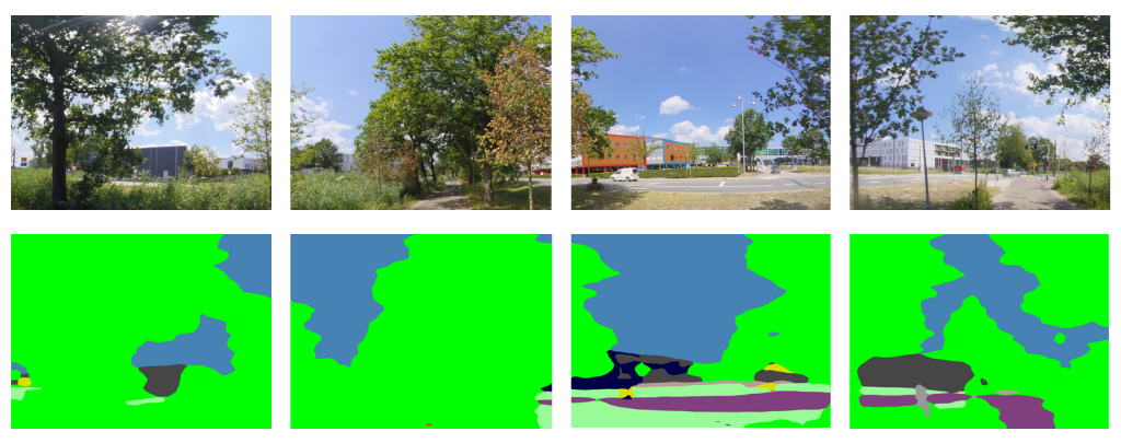
Urban green spaces provide various benefits, but assessing their visibility is challenging. Traditional methods and Google Street View (GSV) has limitations, therefore integrating Volunteered Street View Imagery (VSVI) platforms like Mapillary has been proposed. Mapillary offers open data and a large community of contributors, but it has its own limitations in terms of data quality and coverage. However, for areas with insufficient street image data, the Normalised Difference Vegetation Index (NDVI) can be used as an alternative indicator for quantifying greenery. While some studies have shown the potential of Mapillary for evaluating urban greenness visibility, there is a lack of systematic evaluation and standardised methodologies.
The primary objective of this project is to develop a scalable and reproducible framework for leveraging Mapillary street-view image data to assess the Green View Index (GVI) in diverse geographical contexts. Additionally, the framework will utilise NDVI to supplement information in areas where data is unavailable.
- Setting up the environment
- Explaining the Pipeline
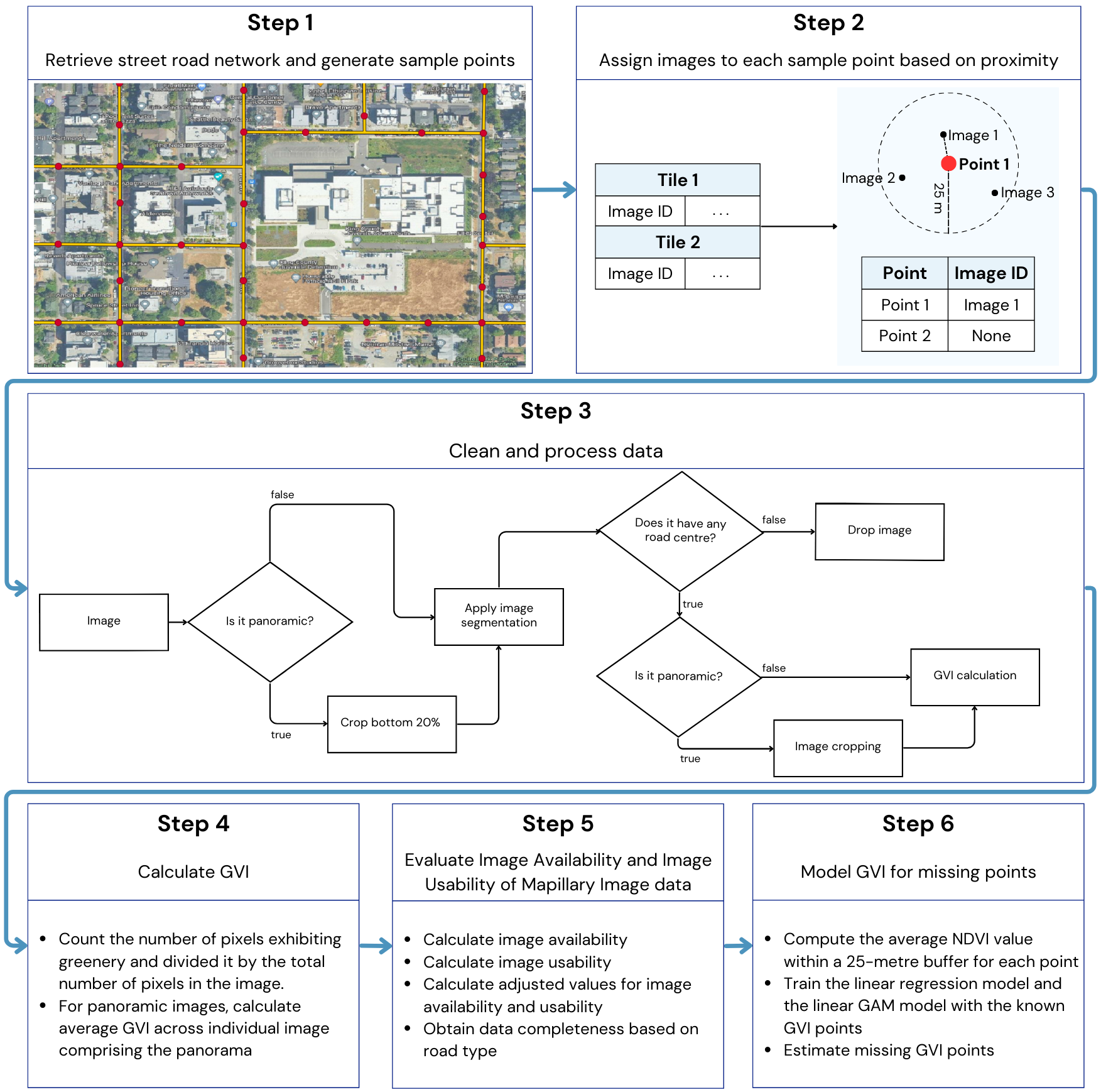
- Step 1. Retrieve street road network and generate sample points
- Step 2. Assign images to each sample point based on proximity
- Step 3. Clean and process data
- Step 4. Calculate GVI
- Step 5 (Optional). Evaluate image availability and image usability of Mapillary Image data
- Step 6 (Optional). Model GVI for missing points
- Acknowledgements and Contact Information
To run the project in Google Colab, you have two options:
- Download the mapillary_GVI_googlecolab.ipynb notebook and open it on Google Colab.
- Alternatively, you can directly access the notebook using this link
Before running the Jupyter Notebook, it is optional but highly recommended to configure Google Colab to use a GPU. Follow these steps:
- Go to the "Runtime" menu at the top.
- Select "Change runtime type" from the dropdown menu.
- In the "Runtime type" section, choose "Python 3".
- In the "Hardware accelerator" section, select "GPU".
- In the "GPU type" section, choose "T4" if available.
- In the "Runtime shape" section, select "High RAM".
- Save the notebook settings
This notebook contains the following code:
- Install Required Libraries: To begin, the notebook ensures that the required libraries are installed, making sure that all the necessary dependencies are available for execution within the Google Colab environment.
%pip install transformers==4.29.2
%pip install geopandas=0.12.2
%pip install torch==1.13.1
%pip install vt2geojson==0.2.1
%pip install mercantile==1.2.1
%pip install osmnx==1.3.0
- Mount Google Drive: To facilitate convenient access to files and storage, the notebook proceeds to mount Google Drive. This step allows for the seamless uploading of the project folder, which can then be easily accessed and utilised throughout the entirety of the notebook.
from google.colab import drive

drive.mount('/content/drive')

%cd /content/drive/MyDrive
- Clone GitHub Repository (If Needed): To ensure the availability of the required scripts and files from the "StreetView-NatureVisibility" GitHub repository, the notebook first checks if the repository has already been cloned in the Google Drive. If the repository is not found, the notebook proceeds to clone it using the 'git clone' command. This step guarantees that all the necessary components from the repository are accessible and ready for use.
import os

if not os.path.isdir('StreetView-NatureVisibility'):
  !git clone https://github.com/Spatial-Data-Science-and-GEO-AI-Lab/StreetView-NatureVisibility.git

%cd StreetView-NatureVisibility
- Set Analysis Parameters: To customise the analysis, it is essential to modify the values of the following variables based on your specific requirements.
place = 'De Uithof, Utrecht'
distance = 50
cut_by_road_centres = 0
access_token = 'MLY|'
file_name = 'utrecht-gvi'
max_workers = 6
num_sample_images = 10
begin = None
end = None
In this example, the main_script.py file will be executed to analyse the Green View Index for De Uithof, Utrecht (Utrecht Science Park).
Replace the following parameters with appropriate values:
- place: indicates the name of the place that you want to analyse. You can set the name of any city, neighbourhood or street you want to analyse.
- distance: Represents the distance between sample points in metres.
- cut_by_road_centres: 1 indicates that panoramic images will be cropped using the road centres. If 0 is chosen, then the panoramic images will be cropped into 4 equal-width images that will allow to analyse the complete panorama.
- access_token: Access token for Mapillary (e.g. MLY|). If you don't have an access token yet, you can follow the instructions on this webpage.
- file_name: Represents the name of the CSV file where the points with the GVI (Green View Index) value will be stored.
- max_workers: Indicates the number of threads to be used. A good starting point is the number of CPU cores in the computer running the code. However, you can experiment with different thread counts to find the optimal balance between performance and resource utilisation. Keep in mind that this may not always be the maximum number of threads or the number of CPU cores.
- num_sample_images: Number of images that are going to be stored along with their segmentations.
- begin and end: Define the range of points to be analysed. If desired, you can omit these parameters, allowing the code to run for the entire dataset. However, specifying the range can be useful, especially if the code stops running before analysing all the points.
- Retrieve Green View Index (GVI) Data: The notebook executes a script ('main_script.py') to retrieve the Green View Index (GVI) data. The script takes the specified analysis parameters as input and performs the data retrieval process.
command = f"python main_script.py '{place}' {distance} {cut_by_road_centres} '{access_token}' {file_name} {max_workers} {begin if begin is not None else ''} {end if end is not None else ''}"
!{command}
- Generate GeoPackage Files (Optional): After retrieving the GVI data, the notebook executes another script ('get_gvi_gpkg.py') to generate GeoPackage files from the obtained CSV files. The generated GeoPackage files include the road network of the analysed place, sample points, and the CSV file containing GVI values.
command = f"python get_gvi_gpkg.py '{place}'"
!{command}
- Compute Mean GVI per Street, and Get Availability and Usability Scores (Optional): Additionally, the notebook provides the option to compute the mean Green View Index (GVI) value per street in the road network. Running a script ('mean_gvi_street.py') achieves this computation.
command = f"python mean_gvi_street.py '{place}'"
!{command}
Once this script was executed, the code to calculate the Image Availability Score and Image Usability Score, along with other quality metrics can be run.
command = f"python results_metrics.py '{place}'"
!{command}
- Estimate missing GVI points with NDVI (Optional): Finally, it is possible to make an estimation of the GVI values for the points that have missing images using the NDVI value and linear regression. Before proceeding to the next cell, please make sure to follow these steps:
- Choose a projection in metres that is suitable for your study area.
- Ensure that you have created the required folder structure: StreetView-NatureVisibility/results/{place}/ndvi.
- Place the corresponding NDVI file, named ndvi.tif, inside this folder. It is recommended to use an NDVI file that has been consistently generated for the study area over the course of a year. The NDVI file must be in the same chosen projection for your area of study
Important note: please note that the EPSG code specified in the code, which is 32631, is just an example for De Uithof, Netherlands.
epsg_code = 32631
command = f"python predict_missing_gvi.py '{place}' {epsg_code} {distance}"
!{command}
- Accessing Results: Once the analysis is completed, you can access your Google Drive and navigate to the 'StreetView-NatureVisibility/results/' folder. Inside this folder, you will find a subfolder named after the location that was analysed. This subfolder contains several directories, including:
- roads: This directory contains the road network GeoPackage file, which provides information about the road infrastructure in the analysed area.
- points: Here, you can find the sample points GeoPackage file, which includes the spatial data of the sampled points used in the analysis.
- ndvi: This directory has the GeoPackage file with the estimated GVI values using linear regression.
- gvi: Initially, this directory contains the CSV file generated during the analysis. It includes the calculated Green View Index (GVI) values for each sampled point. Additionally, if the script for computing the mean GVI per street was executed, this directory will also contain a GeoPackage (GPKG) file with the GVI values aggregated at the street level.
To create a Conda environment and run the code using the provided YML file, follow these steps:
- Cloning GitHub Repository: Open a terminal or command prompt on your computer and navigate to the directory where you want to clone the GitHub repository using the following commands:
- Use the cd command to change directories. For example, if you want to clone the repository in the "Documents" folder, you can use the following command:
cd Documents - Clone the GitHub repository named "StreetView-NatureVisibility" by executing the following command:
git clone https://github.com/Spatial-Data-Science-and-GEO-AI-Lab/StreetView-NatureVisibility.git
This command will download the repository and create a local copy on your computer.
- Once the cloning process is complete, navigate to the cloned repository by using the cd command:
cd StreetView-NatureVisibility
- Use the cd command to change directories. For example, if you want to clone the repository in the "Documents" folder, you can use the following command:
- Create a Conda environment using the provided YML file: Run the following command to create the Conda environment:
conda env create -f mapillaryGVI.yml
This command will read the YML file and start creating the environment with the specified dependencies. The process may take a few minutes to complete.
- Activate conda environment: After the environment creation is complete, activate the newly created environment using the following command:
conda activate mapillaryGVI
- Compute GVI index: Once the environment is activated, you can start using the project. To run the code and analyse the Green View Index of a specific place, open the terminal and execute the following command:
python main_script.py place distance cut_by_road_centres access_token file_name max_workers num_sample_images begin end
Replace the following parameters with appropriate values:
- place: indicates the name of the place that you want to analyse. You can set the name of any city, neighbourhood or street you want to analyse.
- distance: Represents the distance between sample points in metres.
- cut_by_road_centres: 1 indicates that panoramic images will be cropped using the road centres. If 0 is chosen, then the panoramic images will be cropped into 4 equal-width images that will allow to analyse the complete panorama.
- access_token: Access token for Mapillary (e.g. MLY|). If you don't have an access token yet, you can follow the instructions on this webpage.
- file_name: Represents the name of the CSV file where the points with the GVI (Green View Index) value will be stored.
- max_workers: Indicates the number of threads to be used. A good starting point is the number of CPU cores in the computer running the code. However, you can experiment with different thread counts to find the optimal balance between performance and resource utilisation. Keep in mind that this may not always be the maximum number of threads or the number of CPU cores.
- num_sample_images: Number of images that are going to be stored along with their segmentations.
- begin and end: Define the range of points to be analysed. If desired, you can omit these parameters, allowing the code to run for the entire dataset. However, specifying the range can be useful, especially if the code stops running before analysing all the points.
- Generate GeoPackage Files (Optional): After retrieving the GVI data, you have the option to generate GeoPackage files from the obtained CSV files. This step can be executed by running the following command in the terminal:
python get_gvi_gpkg.py place
- Compute Mean GVI per Street, and Get Availability and Usability Scores (Optional): Additionally, you can compute the mean Green View Index (GVI) value per street in the road network. To perform this computation, run the following command in the terminal:
python mean_gvi_street.py place
Once this script was executed, the script to calculate the Image Availability Score and Image Usability Score, along with other quality metrics can be run.
python results_metrics.py place
- Estimate missing GVI points with NDVI file (Optional): Finally, it is possible to make an estimation of the GVI values for the points that have missing images using the NDVI value and linear regression. Before proceeding to the next cell, please make sure to follow these steps:
- Make sure to use an appropriate projection in metres that is suitable for your study area. For example, you can use the same projection as the one used in the roads.gpkg file.
- Ensure that you have created the required folder structure: StreetView-NatureVisibility/results/{place}/ndvi. Place the corresponding NDVI file, named ndvi.tif, inside this folder. It is recommended to use an NDVI file that has been consistently generated for the study area over the course of a year. The NDVI file must be in the same chosen projection for your area of study.
python predict_missing_gvi.py {place} {epsg_code} {distance} - Accessing Results: Once the analysis is completed, you can navigate to the cloned repository directory on your local computer. Inside the repository, you will find a folder named results. Within the results folder, there will be a subfolder named after the location that was analysed. This subfolder contains several directories, including:
- roads: This directory contains the road network GeoPackage file, which provides information about the road infrastructure in the analysed area.
- points: Here, you can find the sample points GeoPackage file, which includes the spatial data of the sampled points used in the analysis.
- ndvi: This directory has the GeoPackage file with the estimated GVI values using linear regression.
- gvi: Initially, this directory contains the CSV file generated during the analysis. It includes the calculated Green View Index (GVI) values for each sampled point. Additionally, if the script for computing the mean GVI per street was executed, this directory will also contain a GeoPackage (GPKG) file with the GVI values aggregated at the street level.
For this explanation, Utrecht Science Park will be used. Therefore, the command should look like this:
python main_script.py 'De Uithof, Utrecht' 50 0 'MLY|' sample-file 8When executing this command, the code will automatically run from Step 1 to Step 4.
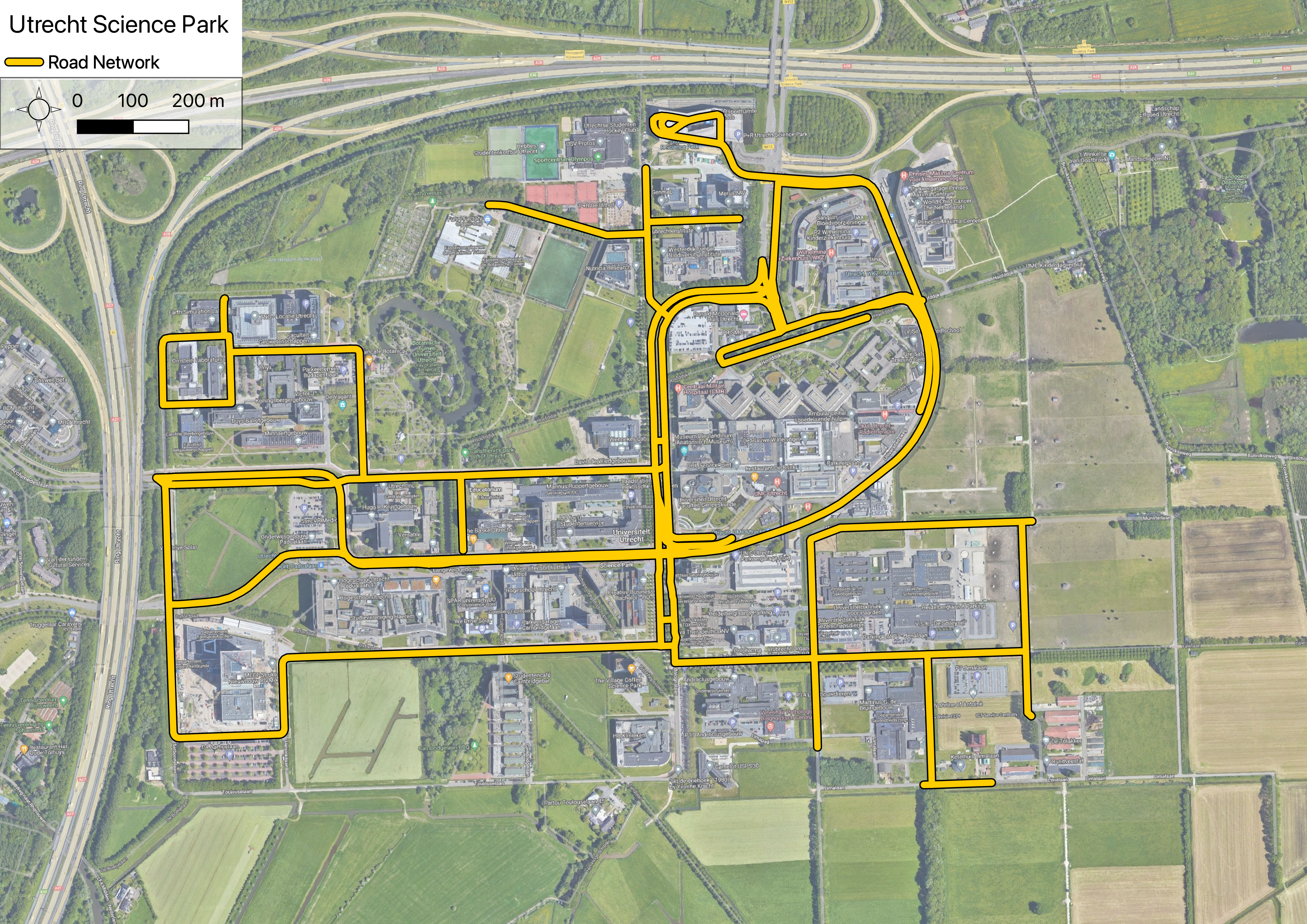
The first step of the code is to retrieve the road network for a specific place using OpenStreetMap data with the help of the OSMNX library. It begins by fetching the road network graph, focusing on roads that are suitable for driving. One important thing to note is that for bidirectional streets, the osmnx library returns duplicate lines. In this code, we take care to remove these duplicates and keep only the unique road segments to ensure that samples are not taken on the same road multiple times, preventing redundancy in subsequent analysis.
Following that, the code proceeds to project the graph from its original latitude-longitude coordinates to a local projection in metres. This projection is crucial for achieving accurate measurements in subsequent steps where we need to calculate distances between points. By converting the graph to a local projection, we ensure that our measurements align with the real-world distances on the ground, enabling precise analysis and calculations based on the road network data.
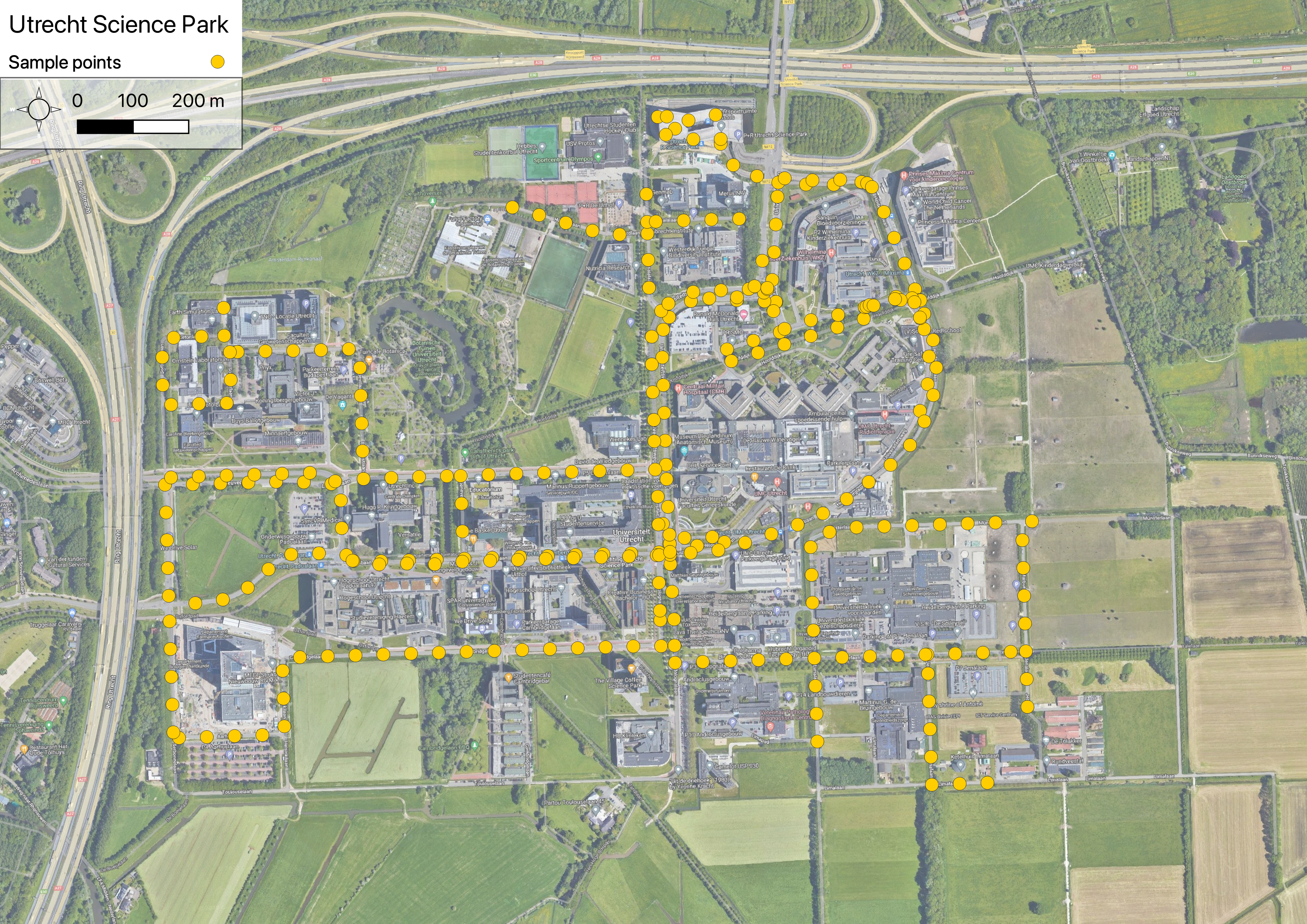
road = get_road_network(place)Then, a list of evenly distributed points along the road network, with a specified distance between each point is generated. This is achieved using a function that takes the road network data and an optional distance parameter N, which is set to a default value of 50 metres.
The function iterates over each road in the roads dataframe and creates points at regular intervals of the specified distance (N). By doing so, it ensures that the generated points are evenly spaced along the road network.
To maintain a consistent spatial reference, the function sets the Coordinate Reference System (CRS) of the gdf_points dataframe to match the CRS of the roads dataframe. This ensures that the points and the road network are in the same local projected CRS, measured in metres.
Furthermore, to avoid duplication and redundancy, the function removes any duplicate points in the gdf_points dataframe based on the geometry column. This ensures that each point in the resulting dataframe is unique and represents a distinct location along the road network.
points = select_points_on_road_network(road, distance)| geometry | |
|---|---|
| 0 | POINT (649611.194 5772295.371) |
| 1 | POINT (649609.587 5772345.345) |
| 2 | POINT (649607.938 5772395.318) |
| 3 | POINT (649606.112 5772445.285) |
| 4 | POINT (649604.286 5772495.252) |
The next step in the pipeline focuses on finding the closest features (images) for each point.
To facilitate this process, the map is divided into smaller sections called tiles. Each tile represents a specific region of the map at a given zoom level. The XYZ tile scheme is employed, where each tile is identified by its zoom level (z), row (x), and column (y) coordinates. In this case, a zoom level of 14 is used, as it aligns with the supported zoom level in the Mapillary API.
The get_features_on_points function utilises the mercantile.tile function from the mercantile library to determine the tile coordinates for each point in the points dataframe. By providing the latitude and longitude coordinates of a point, this function returns the corresponding tile coordinates (x, y, z) at the specified zoom level.
Once the points are grouped based on their tile coordinates, the tiles are downloaded in parallel using threads. The get_features_for_tile function constructs a unique URL for each tile and sends a request to the Mapillary API to retrieve the features (images) within that specific tile.
To calculate the distances between the features and the points, a k-dimensional tree (KDTree) approach is employed using the local projected CRS in metres. The KDTree is built using the geometry coordinates of the feature points. By querying the KDTree, the nearest neighbours of the points in the points dataframe are identified. The closest feature and distance information are then assigned to each point accordingly.
features = get_features_on_points(points, access_token, distance)| geometry | tile | feature | distance | image_id | is_panoramic | id | |
|---|---|---|---|---|---|---|---|
| 0 | POINT (5.18339 52.08099) | Tile(x=8427, y=5405, z=14) | {'type': 'Feature', 'geometry': {'type': 'Poin... | 4.750421 | 211521443868382 | False | 0 |
| 1 | POINT (5.18338 52.08144) | Tile(x=8427, y=5405, z=14) | {'type': 'Feature', 'geometry': {'type': 'Poin... | 0.852942 | 844492656278272 | False | 1 |
| 2 | POINT (5.18338 52.08189) | Tile(x=8427, y=5405, z=14) | {'type': 'Feature', 'geometry': {'type': 'Poin... | 0.787206 | 938764229999108 | False | 2 |
In this step, the download_images_for_points function is responsible for efficiently downloading and processing images associated with the points in the GeoDataFrame to calculate the Green View Index (GVI). The function performs the following sub-steps:
-
Initialisation and Setup: The function initialises the image processing models and prepares the CSV file for storing the results. It also creates a lock object to ensure thread safety during concurrent execution.
-
Image Download and Processing: The function iterates over the rows in the GeoDataFrame and submits download tasks to a ThreadPoolExecutor for concurrent execution. Each task downloads the associated image, applies specific processing steps, and calculates the GVI. The processing steps include:
-
Panoramic Image Cropping using Road Centers: If the image is panoramic and destined for cropping using road centers, the following steps are followed:
- Crop the bottom 20% band to improve analysis accuracy, focusing on critical features.
- Apply semantic segmentation to categorize different regions or objects within the image.
- Augment the panorama's width by wrapping the initial 25% of the image around its right edge. This addition enhances the scene's comprehensiveness.
- Identify road centres using the segmentation output to to establish the base points for cropping.
- Crop the image based on the found road centres.
-
Panoramic Image without Road Center Cropping: When dealing with panoramic images not intended for cropping via road centers, the process unfolds as follows:
- Crop the bottom 20% band to improve analysis accuracy
- Apply semantic segmentation to assign labels to different regions or objects in the image.
- Divide the image into four equal-width sections.
-
Non-Panoramic Image
- Apply semantic segmentation to assign labels to different regions or objects in the image.
- Identify road centres using the segmentation to determine the suitability of the image. This involves ascertaining whether the camera angle captures a valuable portion of the panorama for analysis.
- If road centers cannot be identified, the image is disregarded and excluded from further analysis.
-
results = download_images_for_points(features_copy, access_token, max_workers, place, file_name)After each image is cleaned and processed with previous steps, the Green View Index (GVI), representing the percentage of vegetation visible in the analysed images, is calculated.
The GVI results, along with the is_panoramic flag and error flags, are collected for each image. The results are written to a CSV file, with each row corresponding to a point in the GeoDataFrame, as soon as a thread finishes its task.
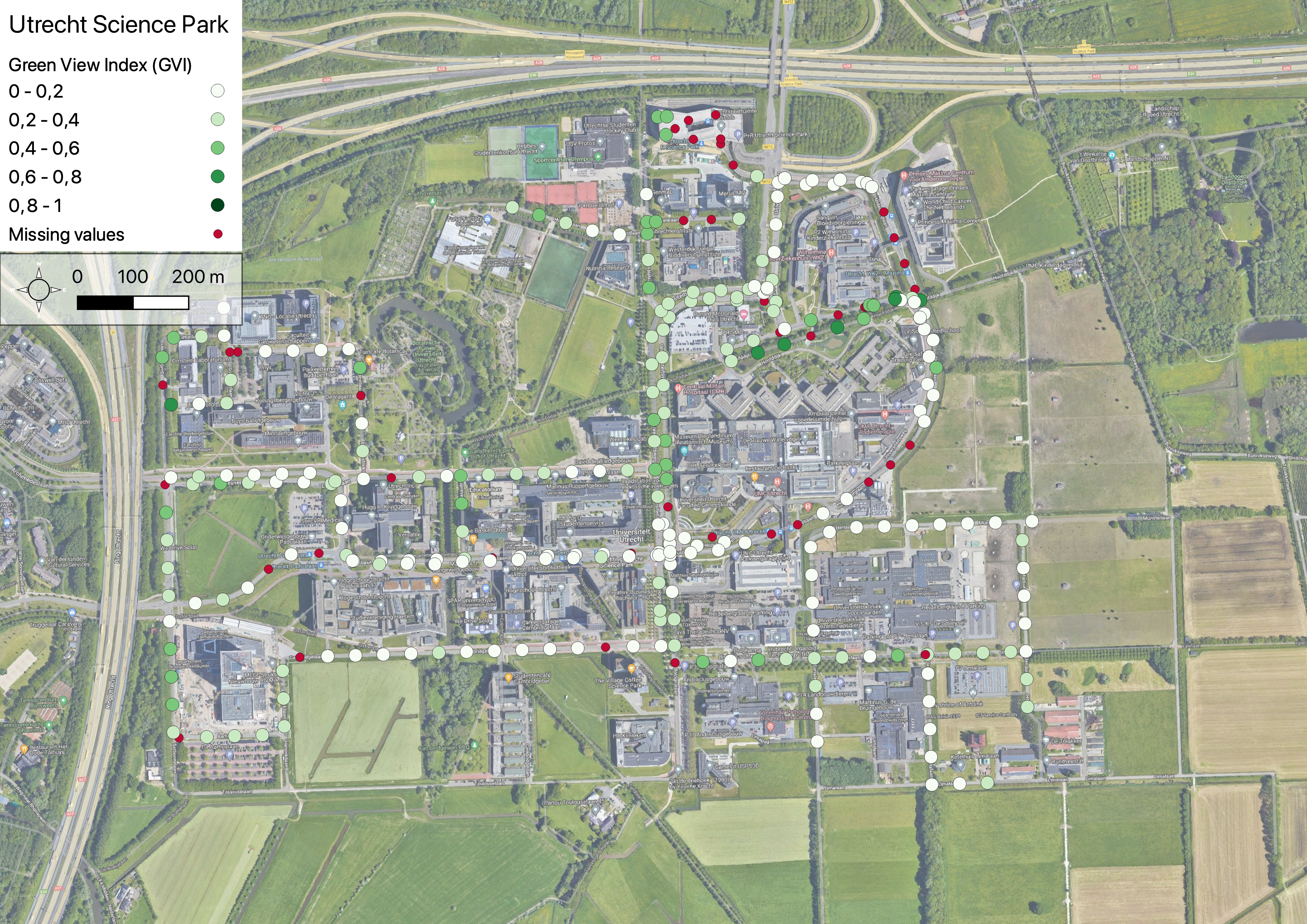
When the code ends running, there will be a folder in "results/{place}/gvi", which will contain a CSV file with the results. We can use it as a GeoDataframe using the following code.
path = "results/De Uithof, Utrecht/gvi/gvi-points.csv"
results = pd.read_csv(path)

# Convert the 'geometry' column to valid Point objects
results['geometry'] = results.apply(lambda row: Point(float(row["x"]), float(row["y"])), axis=1)

# Convert the merged DataFrame to a GeoDataFrame
gdf = gpd.GeoDataFrame(results, geometry='geometry', crs=4326)After analysing the desired images, the image availability and usability are measured by utilising the following equations:
Then, to allow comparisons between multiple cities, the adjusted scores for both metrics are calculated by multiplying the natural logarithm of the road length.
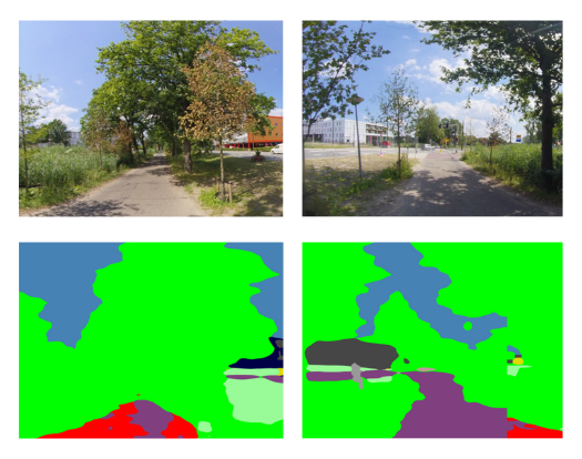
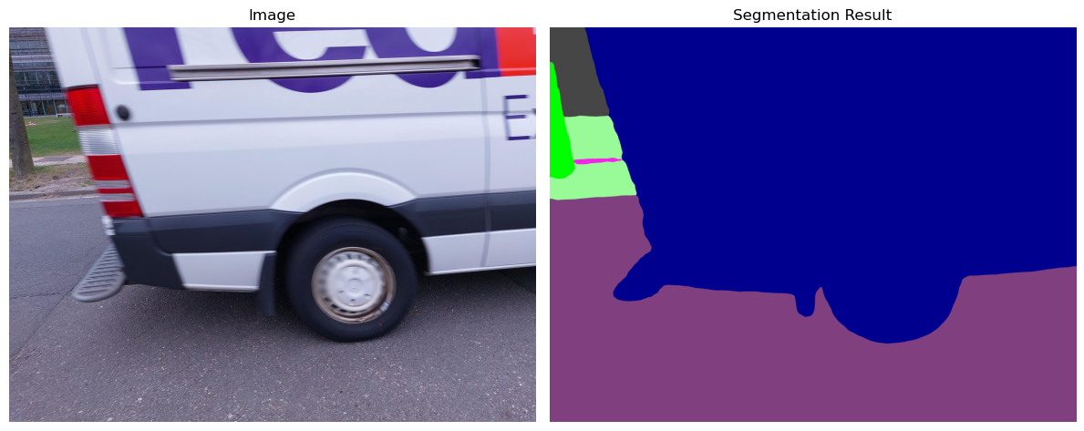
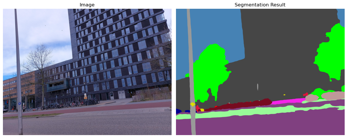
python results_metrics.py "De Uithof, Utrecht"To illustrate the types of images considered usable for this analysis, we provide the following examples. As it can be seen, the images that are centred on the road are deemed suitable for this analysis. However, images with obstructed or limited visibility have been excluded due to their lack of useful information. This selection was made using the algorithm developed by Matthew Danish.
Suitable images for the analysis
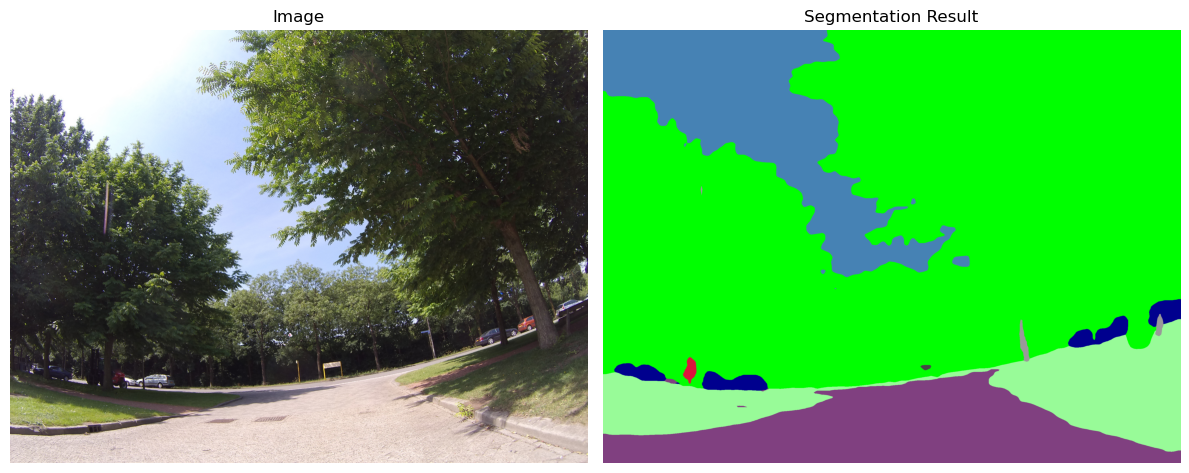

Unsuitable images for the analysis
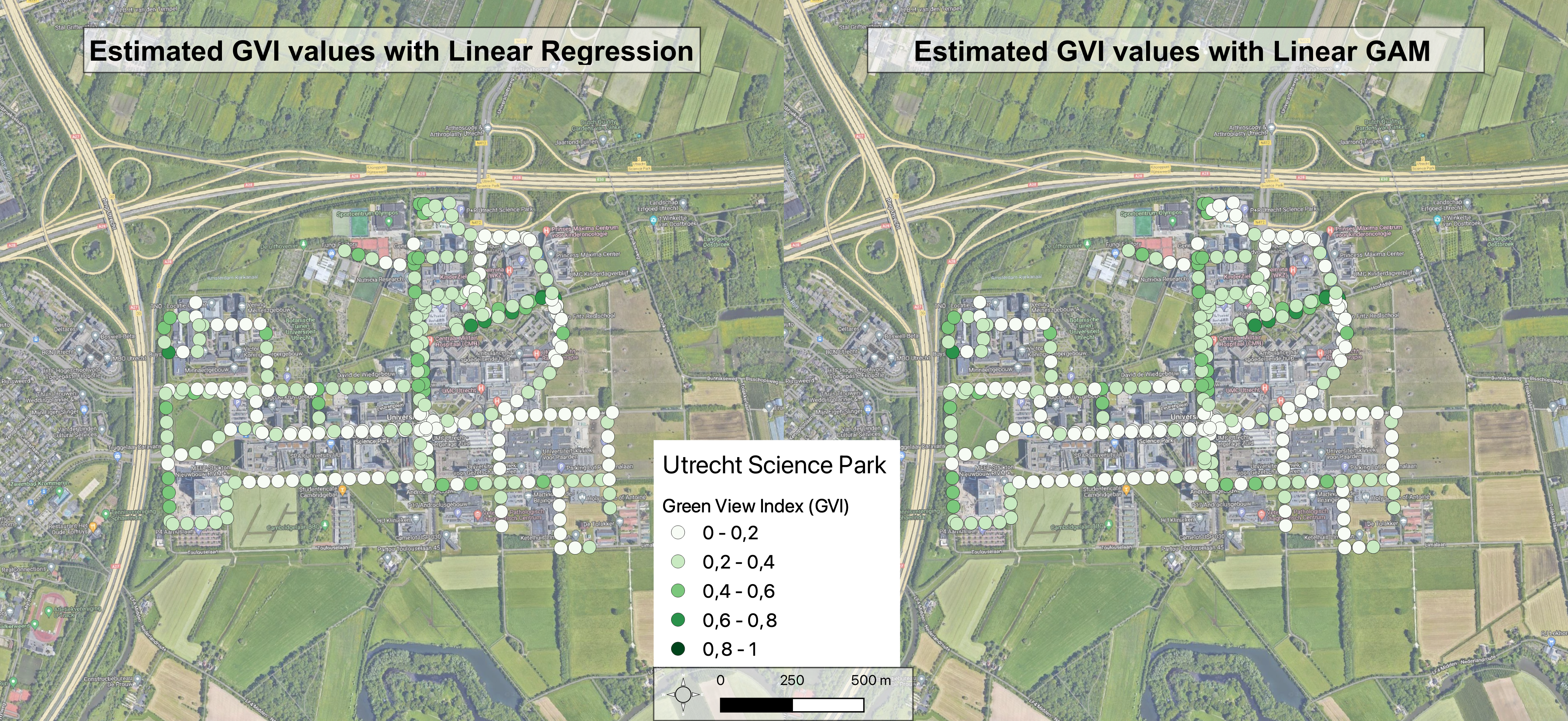
Finally, the analysis employs Linear Regression and Linear Generalised Additive models (GAM) to extract insights from the GVI points calculated in the previous step. The primary objective here is to estimate the GVI values for points with missing images. For this purpose, the code incorporates a module developed by Yúri Grings, which facilitates the extraction of the NDVI values from a TIF file for a given list of points of interest.
To successfully execute this step, an NDVI file specific to the study area is needed. For optimal results, it is recommended to use an NDVI file that has been consistently generated for the study area throughout an entire year. Furthermore, ensure that the coordinate reference system (CRS) of the NDVI file is projected, with metres as the unit of measurement.
python predict_missing_gvi.py "De Uithof, Utrecht" 32631 50| Linear Regression | Linear GAM | |
|---|---|---|
| RMSE | 0.1707 | 0.1640 |
| AIC | -879.7232 | -899.8143 |
Project made in collaboration with Dr. SM Labib from the Department of Human Geography and Spatial Planning at Utrecht University. This is a project of the Spatial Data Science and Geo-AI Lab, conducted for the Applied Data Science MSc degree
Ilse Abril Vázquez Sánchez
i.a.vazquezsanchez@students.uu.nl
GitHub profile: iabrilvzqz
Dr. S.M. Labib
s.m.labib@uu.nl
