sadj

The sadj package allows for relatively flexible use of the underlying X13-ARIMA-SEATS program.

Copyright and Licensing

This document is Crown copyright (c) 2021, Statistics New Zealand on behalf of the New Zealand Government, and is licensed under the Creative Commons Attribution 4.0 International License. To view a copy of this license, visit http://creativecommons.org/licenses/by/4.0/ or send a letter to Creative Commons, PO Box 1866, Mountain View, CA 94042, USA.

Single Series

Results can be produced quickly and easily by accepting default parameters. Consider the following:

ap <- X13Series(AirPassengers)

This produces an object, ap, of class X13Series. This object is initialised with the built-in AirPassengers object–a time series holding the classic Box and Jenkins airline passengers data. Once imported, the data is coerced into a data.frame which looks as follows:

head(ap, 10)

date	year	period	value
1949-01-01	1949	1	112
1949-02-01	1949	2	118
1949-03-01	1949	3	132
1949-04-01	1949	4	129
1949-05-01	1949	5	121
1949-06-01	1949	6	135
1949-07-01	1949	7	148
1949-08-01	1949	8	148
1949-09-01	1949	9	136
1949-10-01	1949	10	119

In fact, while we provide the ability to create an X13Series object directly from a ts object because it is a commonly used type in R, we can also create one from a data.frame like the one displayed above.

An X13Series object has a number of attributes stored interally, such as the adjustment specifications required by the X13-ARIMA-SEATS program. For example, the specifications are held in an attribute called SpecList, and can be retrieved via getSpecList(ap):

getSpecList(ap)

series{
  save=(b1)
}

x11{
  mode=mult
  sigmalim=(1.8,2.8)
  save=(d8 d10 d11 d12 d13 c17)
}

The specification is actually an R list, but it has a print method that displays a familiar string representation. In this case, a default, minimal specification was provided, but there are facilities for providing different specifications when creating X13Series objects, or modifying specifications for existing objects. The details of working with specifications are outlined in a vignette, vignette("specifications", package = "sadj").

In this simple example, no adjustment specifications were explicitly provided. In actual fact, though, a default specification was provided, and the original call to X13Series could have been written in the following equivalent way:

ap1 <- X13Series(AirPassengers, type = "x11")

If the SEATS adjustment method is preferred over X11, then a default SEATS adjustment is also readily available:

ap2 <- X13Series(AirPassengers, type = "seats")
getSpecList(ap2)

series{
  save=(b1)
}

transform{
  function=auto
}

automdl {}

seats{
  save=(s10 s11 s12 s13 s14 s16 s18 cyc ltt)
}

Seasonal adjustment is carried out by calling adjust on an adjustable object:

ap.res <- adjust(ap)

The result in this case is of class X13SeriesResult. It is a data frame containing the raw series and X13-ARIMA-SEATS output tables such as d10, d11, and d12 as columns:

head(ap.res, 10)

date	year	period	value	b1	c17	d10	d11	d12	d13	d8
1949-01-01	1949	1	112	112	1	0.9032879	123.9915	125.1880	0.9904425	0.8958401
1949-02-01	1949	2	118	118	1	0.9387842	125.6945	125.5189	1.0013992	0.9411153
1949-03-01	1949	3	132	132	1	1.0588508	124.6635	125.7773	0.9911445	1.0499907
1949-04-01	1949	4	129	129	1	0.9942750	129.7428	125.9183	1.0303728	1.0246508
1949-05-01	1949	5	121	121	1	0.9767154	123.8846	125.9227	0.9838144	0.9610430
1949-06-01	1949	6	135	135	1	1.0717429	125.9630	125.9575	1.0000438	1.0720059
1949-07-01	1949	7	148	148	1	1.1789500	125.5354	126.2282	0.9945114	1.1724746
1949-08-01	1949	8	148	148	1	1.1760639	125.8435	126.6648	0.9935162	1.1677522
1949-09-01	1949	9	136	136	1	1.0638393	127.8389	127.2535	1.0045996	1.0672713
1949-10-01	1949	10	119	119	1	0.9167217	129.8104	127.9213	1.0147676	0.9288268

In fact, any output produced by X13-ARIMA-SEATS that is a time series is added as a column to the output data frame. The columns can vary depending on the adjustement specification and, besides, are somewhat esoteric. For this reason, helper functions exist for extracting the more common components of an adjusted series in a more uniform way. For example, the raw, seasonally adjusted and trend series can be accessed by calling actual, seasadj, and trend, respectively.

head(trend(ap.res), 10)

year	period	trend
1949	1	125.1880
1949	2	125.5189
1949	3	125.7773
1949	4	125.9183
1949	5	125.9227
1949	6	125.9575
1949	7	126.2282
1949	8	126.6648
1949	9	127.2535
1949	10	127.9213

Output that isn’t a times series is stored as an attribute. For example, the ‘UDG’ file, if present, is a file containing a range of summary statistics and the like, and is read in as a list and stored as an attribute called udg. Many of these attributes aren’t directly useful, and helper functions are instead provided which give the appropriate access. 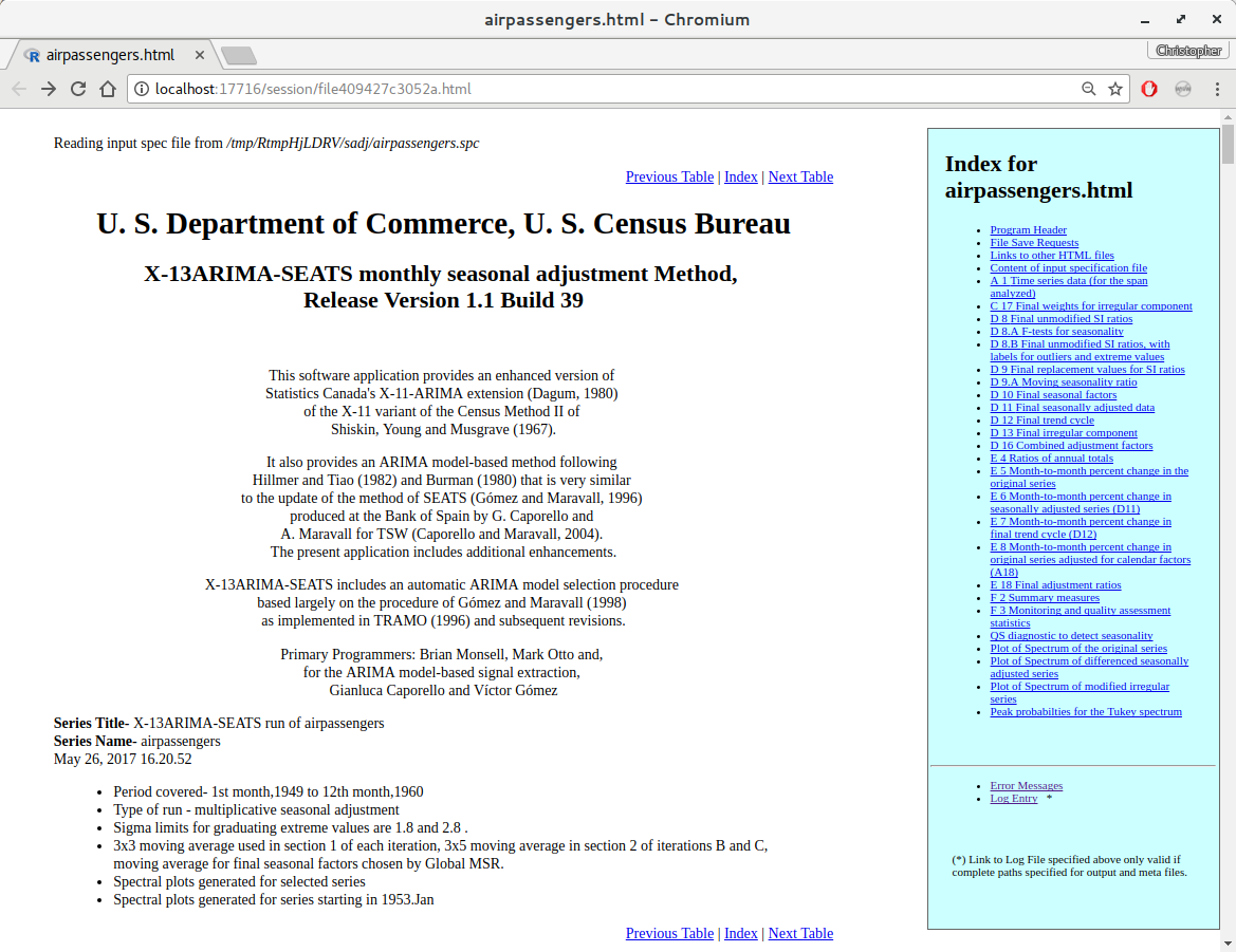For example, calling summary on an adjusted series will cause the HTML version of the output to display, or else it will cause a relatively pretty tabular version of the udg attribute to display:

summary(ap.res, html = TRUE)

or:

summary(ap.res)

stat	value
f2.mcd	3
f2.ic	1.34
f2.is	3.10
f2.fsd8	186.047 0.00
f2.msf	2.705 0.38
f3.m01	0.106
f3.m02	0.104
f3.m03	0.169
f3.m04	0.643
f3.m05	0.315
f3.m06	0.362
f3.m07	0.202
f3.m08	0.354
f3.m09	0.309
f3.m10	0.379
f3.m11	0.346
f3.q	0.27
f3.qm2	0.29

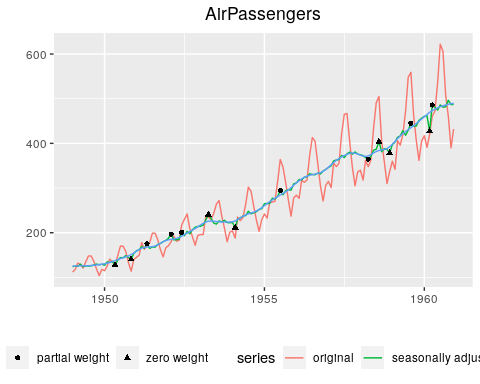
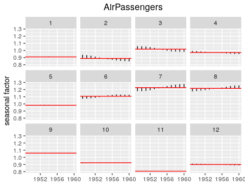
There are a range of built-in plotting functions provided to visualise the results:

plot(ap.res)

plot(ap.res, type = "d10")

Batch Series

The first thing you might want to do is run seasonal adjustment on your existing X13-ARIMA-SEATS file setup and evaluate the results. You might do something like the following:

1.) Read the series batch in from an .mta file:

mta_path <- "~/Network-Shares/corp-nas/seasadj/hlfs/hlfs.mta"
hlfs <- X13BatchFromMTA(mta_path)

2.) Seasonally adjust the series batch:

hlfs_res <- adjust(hlfs)

3.) View summary information of the result:

print(hlfs_res)
summary(hlfs_res)

# Print T-vals of regressors
tvals(hlfs_res)

Interrogate

4.) Interrogate specific series from the batch

library(magrittr) # for pipes

# Use the snames from print/summary of the batch result to plug into `selectSeries`:
munemp_res <- hlfs_res %>% selectSeries("munemp")

# Spin up a Shiny to view plots and diagnostics
munemp_res %>% view()

# View summary diagnostic information
munemp_res %>% summary()

# View full html diagnostic report
munemp_res %>% summary(html=TRUE)

# What plots are there?
?sadj:::plot.X13SeriesResult

# Try a plot
munemp_res %>% plot(type="D10D8")

# How about an interactive plot?
munemp_res %>% plot(type="D10D8", interactive = TRUE)

5.) Interrogate an entire batch

# Query Specs

# getParamVals.X13Batch
res <- getParamVals(hlfs,"series","span") %>% map( ~.x[[1]])

# getSpecParameter.X13Batch
# Same as getParamVals but it doesn't try to parse individual values
# Example of querying documenation
?sadj:::getSpecParameter.X13Batch

Update/Modify

6.) Update/Modify an entire batch

# Modify Specs

# Add/remove outliers
# Add a Level shift to all series in a batch
# (Try querying to verify this)
addOutliers(hlfs) <- "LS2020.2"

# Remove the level shift
removeOutliers(hlfs) <- "LS2020.2"
# By default, removeOutliers does not clear out the save argument
# That is something to be fixed, but for now:
setSpecParameter(hlfs, "regression", "save") <- NULL

# Add outliers to a subset of series:
setSpecParameter(hlfs
                 , snames = c("munemp", "funemp")
                 ,"regression", "variables") <- c("LS1980.3")

Sadj objects Summary

Input Objects

Object	Structure	Comments
X13Batch	A list of X13SeriesGroup objects	A batch of X13Series objects as specified by an MTA file.
X13SeriesGroup	A list of X13Series objects	X13Series object groupings which are delineated by empty spaces inside an MTA file (see note). Either 0 or 1 composites are allowed at the end of a group and nowhere else.
X13Series	A dataframe of time series data	Can have several attributes to represent the following X13 files that can be associated with a single series: spc, fac, regression. Read the X13Series section to learn how to access and modify these attributes

Output Objects

Object	Structure	Comments
X13SeriesResult	A dataframe of seasonally adjusted time series data	Has attributes that represent quality diagnostics and calculated modelling parameters
X13SeriesGroupResult	A list of X13SeriesResult objects	X13SeriesResult object groupings which are delineated by empty spaces inside an MTA file (see note). Either 0 or 1 composites are allowed at the end of a group and nowhere else.
X13BatchResult	A list of X13SeriesGroupResult objects	A batch of X13SeriesResult objects as specified by an MTA file.

Note: Empty lines in an MTA file do not mean anything to the X13 program. They are a Statistics NZ convention and they do mean something to the sadj package - The groupings are submitted to X13 as their own batches.

Interacting with Objects

Modifying Seasonal Adjustment Congfigurations (SPC files)

X13Series is a dataframe with time series input data. It has attributes that are accessible/mutable with the following functions:

get	set	comments
getSpecList	setSpecList	Method gets passed to the X13SpecList object which is attached to X13Series as an attribute
getSpec	setSpec	Same as comment above
getSpecParameter	setSpecParameter	Same as comment above
getFacFile	setFacFile	get/set the factor file dataframe attached to the the X13Series
getRegFile	setRegFile	get/set the regression file dataframe attached to the the X13Series

StatisticsNZ/sadj