Abstract: The last decade has witnessed tremendous progress in deep learning classification tasks; however, these models often rely on a notable “closed-set assumption”: that classes observed in test-time are a subset of those observed during train-time. We present a new method, called Novel-Net, which integrates Gaussian Mixture Models into an arbitrary deep network architecture to discriminate instances not seen during training time. Our model consistently outperforms conventional techniques such as Nearest-Class Mean and Model Confidence, boosting accuracy by 12% in binary classification tasks.
| K-Means | Gaussian Mixture Models |
|---|---|
 |
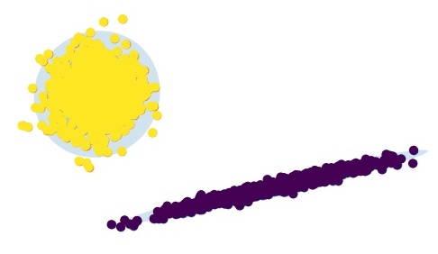 |
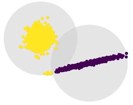
Figure 1. Classification of two distributions using K-Means and Gaussian Mixture Models that demonstrates the relative flexibility of the latter framework.
Image classification has made significant progress since the incorporation of Neural Network approaches. However, a common assumption many models make is that at test-time the set of classes encountered would be a subset of all the classes the model observed at train-time [5]. In other words, Neural Networks do not know what they do not know.
Consider the case of an automated diagnostician agent trained on samples of k distinct pathologies. At test-time the agent should not only correctly distinguish between corresponding test samples, but ideally identify unfamiliar samples and signal caution. In this example, the agent’s ability to identify novel samples could make the difference in discovering a new variant of a highly infectious virus, or simply avoiding a diagnosis with incomplete information. For high-risk deployment, machine learning models must competently acknowledge their limits and drop the assumption that classes seen at test-time are a subset of those observed during train-time.
We are not the first to consider the problem of Open Set Recognition (OSR), and benefit from work spanning both traditional ML and deep learning disciplines. In that spirit, we integrate deep learning architectures with Gaussian Mixture Models (GMMs), which fit inputs to a predetermined number of normal distributions. We opt for GMMs since they have an intuitive notion of distance which still preserves complex relationships in the data. For clarification,consider the scenario shown in Figure 1.
Gaussian Mixture Models are by no means universal approximators [8], but their descriptive flexibility exceeds that of a strict K-Means method [18]. In addition, their decisions are fundamentally explainable, which may be prioritized in high-impact contexts. The greatest theoretical hurdle—and the crux of our work here—is whether the feature space can be meaningfully approximated by a computationally acceptable number of Gaussian clusters. In short, we seek to identify and reject samples from some novel class, N, ideally without compromising model performance. For the sake of this paper, we consider perfor- mance in terms of standard accuracy and measure detection of N by novel-class recall.
Reviews of Open Set Recognition (OSR) and Open World Learning (OWL) typically partition the input space into four quadrants [6, 9, 17]:
- Known-known classes (KKCs): traditional data samples, seen at train time and exemplify one of k classes.
- Known-unknown classes (KUCs): negative data samples defined by a lack of positive instances from other classes; i.e, background classes (think object detec- tion [10]).
- Unknown-known classes (UKCs): Classes with no available data samples during training, but with avail- able semantic information.
- Unknown-unknown classes (UUCs): Classes not encountered during training and also lack semantic in- formation. Essentially, these are data instances that are completely unexpected.
Our work largely ignores UKCs which are a focus in Zero-Shot Learning: a process which leverages similari- ties between KKC and UKC attributes to classify UKC in- stances [6, 19]. Rather, our approach leverages contrasts between KKC and UUC attributes to discriminate the lat- ter samples; i.e, that known class features and unknown class features will be notably distinct. On first glance, OSR resembles prior work on classification with a reject option [6, 7]; however, these frameworks still operate un- der the closed-set assumption—that all instance classes are seen during train-time (KKCs). Since there is substantial overlap between model confi- dence and OSR, we review common methods here. These techniques can be organized into ambiguity-based and dis- tance-based frameworks [7]. Ambiguity-methods reject in- stances whose model probability outputs are within some δ distance from one another [14], as shown in Figure 2. The problem is formally defined assuming a predeter- mined reject-penalty, d, and probability function η [7]:
Conversely, Distance-methods reject samples by thresh- olding some notion of distance between instances and target classes [6, 14]. As the authors mention in [6], empirically setting a threshold value inherently relies upon information determined from KKCs at train-time, which jeopardizes our generalizability to UUCs at test-time. Current approaches take inspiration from the k-nearest neighbors algorithm: classes are represented as a concatenation of all corresponding positive samples, which while computationally infeasible performs comparable to state-of-the-art methods [6, 15]. The authors of [15] introduce a similarly-inspired Nearest-Class-Mean (NCM) classifier, which instead represents classes by the mean feature-vector (learned at train-time) of its corresponding positive samples. Both methods rely on a metric of “distance” between instances and means, implemented by the Mahalanobis distance.
Figure 3. Model probability outputs where outputs of ambiguity within $\sigma = 0.20$ are rejected
The Mahalanobis distance differs from Euclidean distance in that it considers the relationship between instances 195 of a distribution. For any two n-dimensional vectors, $ x_1 , x_2 as \in R^n $. Mahalanobis distance can be computed as
where C is the covariance matrix of the distribution [3]. Aside from traditional methods, recent years have witnessed novelty detection using a deep-learning approach. The authors of [2] propose a new layer, denoted Open-Max, which estimates the probability that a given instance is outside the set of KKCs. Specifically, OpenMax adapts the SoftMax layer for the OSR setting where probabilities do not necessarily sum to 1. Interestingly, OpenMax is largely an ambiguity-based method, rejecting instances whose probability outputs do not exceed a confidence value,
Our work consists of unsupervised learning on unlabeled data using a mixture of Gaussians. Each cluster is a multivariate Gaussian with a mean
where
The model is fit by expectation maximization, and the proper number of components can be determined apriori using either the Akaike or Bayesian information criterion [1,16]. The former metric estimates the difference in probabilistic density between the true model,
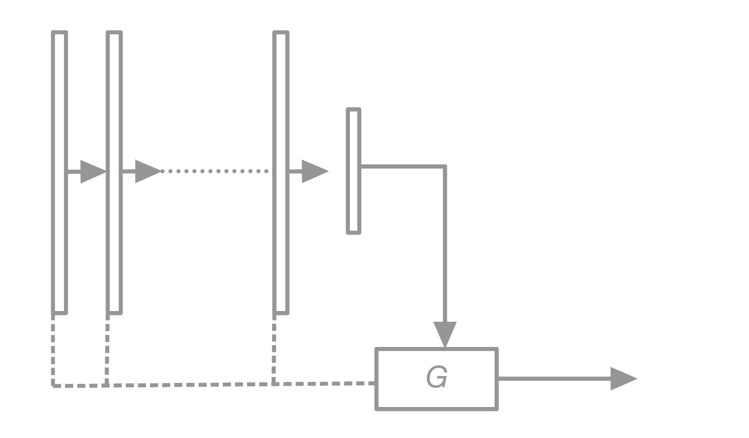
Figure 3. NovelNet “architecture” showing arbitrary an Neural Network and $G$ weed-out component. Dashed lines (- - -) correspond to potential forward feeds into $G$.
To tackle this problem, we propose NovelNet as a new
approach. Figure 3 displays a high-level diagram of Novel-Net, which feeds network features into a
As shown in Figure 3, features may be extracted from any layer. In this manner, our approach draws upon model ambiguity methods, since we may choose to identify patterns directly out of the Softmax layer; however, this raises a prominent question: are unfamiliar Softmax probability relationships indicative of unfamiliar inputs? Ambiguity methods (see Section 2) compare output probabilities at face-value, strictly rejecting instances who “self-report” low confidence. In this work, we consider the probability outputs as any other feature representation. Assuming this hypothesis, we suspect that relationships determined by
Prior to train-time, we specify a max search-space of Gaussian components available (n2 , n3 , ..., nmax ), since computation scales linearly with the number of clusters. Immediately after the network is trained, we extract features from a sample of the training set (the size of which is an ad- 289 justable hyperparameter) and perform a coarse search of the 290 number of components with respect to AIC criterion (see 291 Section 2).
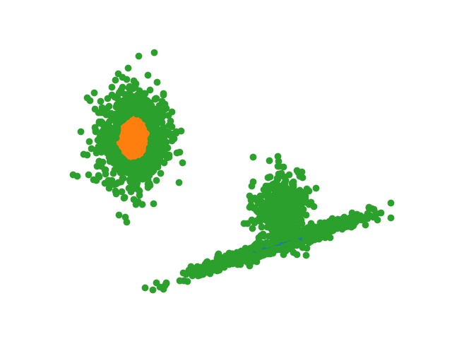
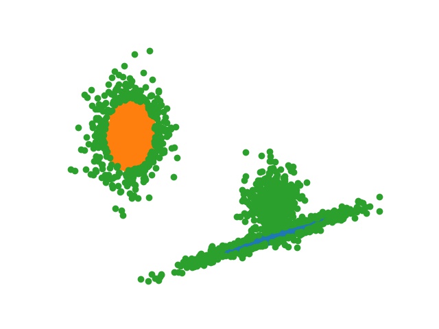
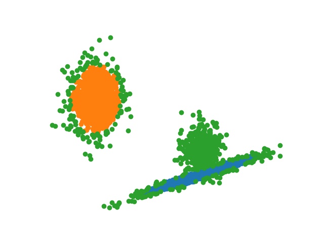
Subsequent to the search, we must identify a maximum distance from the closest cluster, denoted
 |
 |
|---|---|
 |
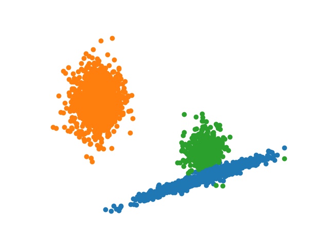 |
Figure 4. Example of increasing the distance threshold across the domain, where green points are UUC instances
As suggested above, each problem approach will be evaluated using essentially the same CNN architecture applied to the CVRC Google Street map dataset. The specifics of each trial’s methodology are described below. Note that due to hardware limitations, all instances have been scaled down to more laptop-friendly 100x100 images.
As a result of hardware limitations, I extract an 11,000 image subset containing an equal mix of Pittsburgh and Orlando instances. Each instance is labeled accordingly, and the model is trained using the architecture shown in Table 1. Panoramic Classification follows nearly the same methodology, except for every point in space (where each point corresponds to 5 images total), we append two images width-wise together, producing a new image of size 3x200x100. These new modified training images are then used to train a near-identical model with slight dimension accommodations listed in the rightmost column. Training will continue over 10 Epochs, and the best model is selected and assessed in the Results section below.
Local Regression discards labels in favor of training directly on the coordinates themselves. A 11, Pittsburgh-image sample is trained on using the L1 loss function, yet apart from these changes, the architecture and methodology remain the same. Training will continue over 10 Epochs, and the best model is selected and assessed in the Results section below.
Partitioned and Clustered Local-Classification will utilize an identical model to that of Conventional Classification; however, applied to the 11,000 sample of Pittsburgh images. In the case of the former, a line will be drawn vertically such that Pittsburgh images to its east will be labeled differently than their neighbors to the west of it. In the case of the latter, we label points only after performing K-Means clustering and evaluating their distance to each centroid, i.e, images in Cluster A will be labeled differently than those in Cluster B. Training will continue over 10 Epochs, and the best model is selected and assessed in the Results section below.
Fig. 4. Accuracy and F1 Evaluation for Macro and Local Classification models
Training evaluation metrics have been tracked by epoch for each classification model (see figure 4) and the best of each is listed in Table 2. Conventional and Panoramic Macro-Classification unsurprisingly outperform all other models; however, it is interesting that the latter both converges faster than and exceeds the former with half the training set size. Unfortunately, this expansion in the feature space came at the cost of added computational burden, and to avoid scaling down the images I migrated the code to Google’s Colab Pro service. Clustered Local Classification consistently outperforms Partitioned Classification by about 4-5%, with negligible computational overhead. Local Regression was largely (and expectedly) a failure: after 10 epochs, the best model predicted coordinate locations with an average L1 error of 0.4◦ which is less impressive than it sounds considering that 0.4◦ spans the entire city of Pittsburgh.
Fig. 5. Model loss (left) alongside example saliency map (right) – the latter [Partition Classification] appears
to take interest in building texture and skylines
A saliency map analysis (example in Figure 5) demonstrates that the local-partition model appears moderately attracted to characteristic structures (i.e skylines, building texture, etc.), though the visual relationship is not overwhelming. More strongly, the model favors human and car elements – suggesting that partitions based on demographic attributes (wealth, ethnicity) may better characterize local geography than architecture. This may suggest that although architectural identity is indeed quite relevant to the trained classification model, so too is the background noise of pixel brightness and general hue.
Fig. 6. Saliency map of Conventional Macro-Classification. The model appears to take interest in both humans
and cars.
I hoped to demonstrate that our approach to a deep learning problem is as critical to success as the architecture itself—that it is as necessary to ask the question of "In what ways can I solve the problem" as "In what ways can I alter the problem". If identifying an image in one of n partitioned cells is the stated goal, it seems unimaginative to overlay an arbitrary boundary when an comparatively learnable one is available. In this paper, the scope of the problem is limited, but we may imagine learned partitions clustered over many potential features of interest (year founded, resident demographics, etc.) such that the application of a CNN is optimal. Compared to a Panoramic feature-extending approach the computational cost is minimal, and its performance benefit is significant. I would like to see (and perform) research which explores this road. Additionally, much of the work done in this paper is done at a small scale utilizing a generic CNN model, yet I’d be curious to analyze the evaluation metrics done on more contemporary architectures; particularly the Inceptio nmodel comes to mind as the visual geolocation problem stands to benefit from a spatially dynamic architecture.
Partly in reaction to recent breakthroughs in neural network research—journalists, academics, and computer scientists continue to voice concern regarding the ongoing deployment of advanced computer vision products. Whether in the hands of stalkers, federal intelligence, or local law enforcement, these technologies have the potential to locate citizens automatically, and as such their use must be vetted by those same citizens.
To Connor O’Brien, who picked up takeout while I worked on this.
[1] Jan Brejcha and Martin Cadik. 2017. State-of-the-art in visual geo-localization.Pattern Analysis and Applications20 ( 2017). https://doi.org/10.1007/s10044-017-0611-
[2] Carl Doersch, Saurabh Singh, Abhinav Gupta, Josef Sivic, and Alexei A. Efros. 2012. What Makes Paris Look like Paris? ACM Trans. Graph.31, 4, Article 101 (jul 2012), 9 pages. https://doi.org/10.1145/2185520.
[3] Ross B. Girshick, Jeff Donahue, Trevor Darrell, and Jitendra Malik. 2013. Rich feature hierarchies for accurate object detection and semantic segmentation.CoRRabs/1311.2524 (2013). arXiv:1311.2524 http://arxiv.org/abs/1311.
[4] Eric Müller-Budack, Kader Pustu-Iren, and Ralph Ewerth. 2018. Geolocation Estimation of Photos using a Hierarchical Model and Scene Classification.
[5] Christian Szegedy, Wei Liu, Yangqing Jia, Pierre Sermanet, Scott E. Reed, Dragomir Anguelov, Dumitru Erhan, Vincent Vanhoucke, and Andrew Rabinovich. 2014. Going Deeper with Convolutions.CoRRabs/1409.4842 (2014). arXiv:1409. http://arxiv.org/abs/1409.
[6] Tobias Weyand, Ilya Kostrikov, and James Philbin. 2016. PlaNet - Photo Geolocation with Convolutional Neural Networks.CoRRabs/1602.05314 (2016). arXiv:1602.05314 http://arxiv.org/abs/1602.
[7] Amir Roshan Zamir and Mubarak Shah. 2014. Image Geo-Localization Based on MultipleNearest Neighbor Feature Matching UsingGeneralized Graphs. IEEE Transactions on Pattern Analysis and Machine Intelligence36, 8 (2014), 1546–1558. https://doi.org/10.1109/TPAMI.2014.


