This repository provides an example of using StochSS Live! to implement a specific epidemiological model and to estimate the parameters for it for a specific county.
StochSS Live! is the web interface for developing and investigating stochastic models found at https://live.stochss.org. All results can be replicated by importing this repositories and notebooks into StochSS Live!.
The libraries used by StochSS Live! for simulation and analysis are a part of the StochSS suite of software.
To install the required libraries from the requirements file, run pip install -r requirements.txt.
- Implementing An Epidemiological Model in StochSS Live!
- Parameter Estimation Workflow using ABC
- References
In the following, we describe the epidemiological model we use, and demonstrate how it can be implemented in the StochSS Live! web interface. Then we describe the process of creating a parameter inference workflow for some local COVID19 data
The epidemiological model we implement is an extended version of the SEIRD model that accounts for symptomatic and asymptomatic cases. The involved compartments (species) are: susceptible (S), exposed (E), infected (I), symptomatic (Y), recovered (R), dead (D), and cleared (C). The system can be visualized as:
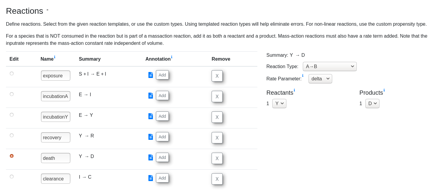
The system evolves according to SEIR dynamics but with a chance of becoming symptomatic after being exposed. We fix the rate at which exposed patients become infectious at 0.16, which represents ~6.25 day incubation period and estimate the proportion of patients who become infected vs. symptomatic. This is roughly adopted from a similar model [5]. Specifically, we have the following set of reactions:
Susceptible + Infected → Infected + Exposed
Exposed → Infected
Exposed → Symptomatic
Symptomatic → Recovered
Symptomatic → Dead
Infected → Cleared
This model assumes that only asymptomatic transmission is possible, all asymptomatic cases recover, and that all parameters are static.
Using this specification, we can implement the model in StochSS Live! in the model creation interface
A pre-implemented version of this model with some default parameters can be found here.
In the model creation interface, we can also preview trajectories if we were to consider the model as either discrete stochastic or an ODE model.
We estimate the parameters of the model for Santa Barbara and Buncombe counties using the Sciope [3] toolbox, part of the StochSS suite of software which offers model exploration and parameter estimation. A pre-implemented template notebook can be generated by using the "Sciope Model Inference" workflow in StochSS Live!.
The completed workflow is included for Santa Barbara, CA and for Buncombe, NC.
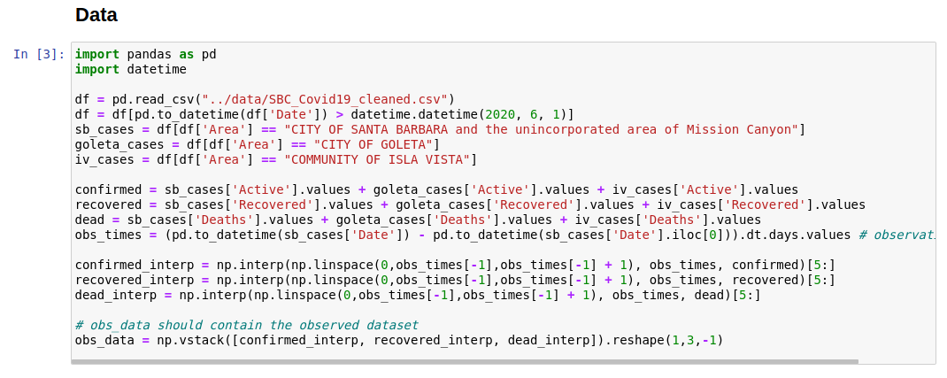
Data for estimating parameters should be loaded in the data block. The
obs_data object should contain the final completed dataset.
Sciope implements various algorithms for Approximate Bayesian Computation [2]. To use these, we need to complete the following segments of the notebook:
- Prior cell
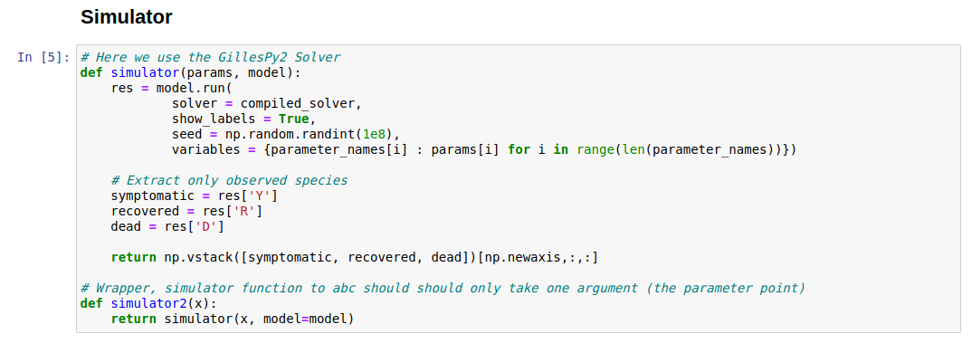
- Simulator function
This function should take in a parameter array and output a simulation from the model that matches the shape of the observed data.
We make one modification because our data consists of observations of the symptomatic, recovered, and dead cases. Therefore, thez output of this function should only return those three species. For SB, this is broken down into these 3 but for Buncombe, we observe cumulative symptomatic and recovered.
- Summary Statistics and Distance Functions
The default algorithm we use is Replenishment ABC-SMC [3]. Sciope uses Dask [4] to parallelize inference so we use the StochSS Live! servers to use more processes.
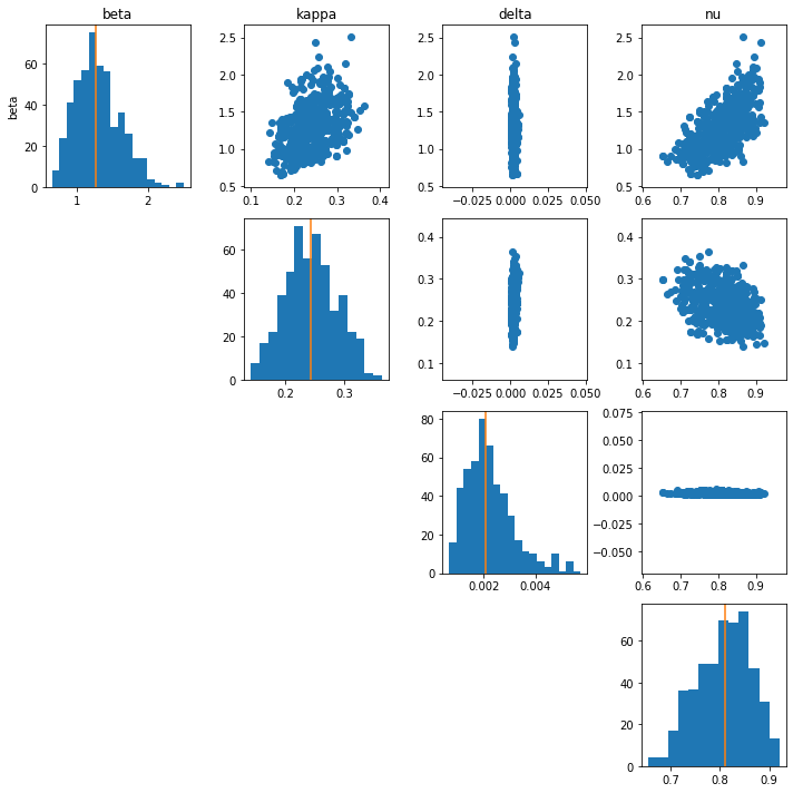
The inference returns a np.array of samples from the the posterior
distribution stored in the posterior object. Each sample can be used
as a set of parameters in the model to generate further trajectories.
Below, we show the posterior distribution of parameters for Santa Barbara as well as generated data from the model using the posterior samples (posterior predictive).
Of importance is that the presented models do not really indicate a sufficient fit to the data to draw any strong conclusions. For a complete analysis, this process needs to be repeated, changing the model to better capture assumptions about the system. For example, we would expect the infectivity to change over time as policies are implemented and we know that there are non-intrinsic measurement error, such as reporting errors in the data.
[1] Prashant Singh, Fredrik Wrede, Andreas Hellander, Scalable machine learning-assisted model exploration and inference using Sciope, Bioinformatics, , btaa673, https://doi.org/10.1093/bioinformatics/btaa673
[2] Sisson, Scott A., Yanan Fan, and Mark Beaumont, eds. Handbook of approximate Bayesian computation. CRC Press, 2018.
[3] C. C. Drovandi and A. N. Pettitt. Estimation of parameters for macroparasite population evolution us-ing approximate Bayesian computation.Biometrics,67(1):225–233, 2011.
[4] Dask Development Team (2016). Dask: Library for dynamic task scheduling URL https://dask.org
[5] Flaxman, S., Mishra, S., Gandy, A. et al. Estimating the effects of non-pharmaceutical interventions on COVID-19 in Europe. Nature 584, 257–261 (2020). https://doi.org/10.1038/s41586-020-2405-7


