Project 2: Traffic Sign Recognition

1. Introduction

The goals / steps of this project are the following:

Load the data set (see below for links to the project data set)
Explore, summarize and visualize the data set
Design, train and test a model architecture
Use the model to make predictions on new images
Analyze the softmax probabilities of the new images
Summarize the results with a written report

2. Project Dependencies

This project requires:

CarND Term1 Starter Kit

3. Data Set Summary & Exploration

3.1 Basic summary of the data set

The code for this step is contained in the code cells 1-3 of the IPython notebook.

I used the numpy and csv library to calculate the summary statistics of the traffic signs data set:

Data Set	#Images	Percentage
Training samples	34799	67.13%
Validation sample	4410	8.51%
Test samples	12630	24.35%

In total the data set consist of 51839 images. Each image has a height x width of 32x32 and 3 color channels (RGB).

The data set contains 43 different German traffic signs as listed below.

ClassId	Signname
0	Speed limit (20km/h)
1	Speed limit (30km/h)
2	Speed limit (50km/h)
3	Speed limit (60km/h)
4	Speed limit (70km/h)
5	Speed limit (80km/h)
6	End of speed limit (80km/h)
7	Speed limit (100km/h)
8	Speed limit (120km/h)
9	No passing
10	No passing for vehicles over 3.5 metric tons
11	Right-of-way at the next intersection
12	Priority road
13	Yield
14	Stop
15	No vehicles
16	Vehicles over 3.5 metric tons prohibited
17	No entry
18	General caution
19	Dangerous curve to the left
20	Dangerous curve to the right
21	Double curve
22	Bumpy road
23	Slippery road
24	Road narrows on the right
25	Road work
26	Traffic signals
27	Pedestrians
28	Children crossing
29	Bicycles crossing
30	Beware of ice/snow
31	Wild animals crossing
32	End of all speed and passing limits
33	Turn right ahead
34	Turn left ahead
35	Ahead only
36	Go straight or right
37	Go straight or left
38	Keep right
39	Keep left
40	Roundabout mandatory
41	End of no passing
42	End of no passing by vehicles over 3.5 metric tons

3.2 Exploratory Visualization of the Dataset

The code for this step is contained in the code cell 6 and 7 of the IPython notebook.

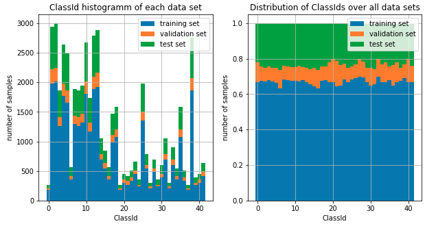
The left bar chart shows the distribution of the traffic sign class IDs for the training, the validation and the test set. The data sets are very unbalanced. E.g. the data sets contains almost 2000 30 km/h speed limit signs but only 180 20 km/h speed limit signs.

As shown in the right chart the data sets well balanced between training, validation and test sets.

The images below give an overview about the German traffic signs contained in the training data set. The image have a huge variation in illumination. Some traffic signs are almost dark. Others are overexposured or show a high reflection (e.g. see the yield signs in the second row).

4. Design and Test a Model Architecture

4.1 Image Pre-Processing and Normalization

The code for this step is contained in the code cell 8 and 9 of the IPython notebook.

As a first step, I decided to convert the images to grayscale because test runs showed almost similar accuracies on the validation set with RGB images. By using grayscale images the input vector can be reduced from 32x32x3 down to 32x32x1. Furthermore, in the specific domain of traffic sign classification, the network looks for characteristic traffic sign structures which can also easily extracted from grayscale images (see also last chapter "visualization of CNN layers").

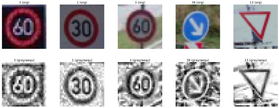
The first row shows the original RGB image while the second row shows the grayscale image.

As a second step, I applied an adaptive histogram equalization in order to improve the contrast especially in the bright and dark images. OpenCV provides the CLAHE (Contrast Limited Adaptive Histogram Equalization) algorithm to exactly achieve this task. The last row in the image above shows the improved images. The "80 km/h speed limit" sign is a good example showing the benefit of this pre-processing step. In the RGB and grayscale image the 80 is almost not visible. After the adaptive histogram equalization the numbers are clearly visible.

As a last step, I normalized the image data to values between -0.5 and 0.5 because the range of input data varies widely (between 0 and 255). Many classifiers are using the euclidean distance in the cost function. If the values vary a lot, the distance will be dominated by these feature. The feature normalization brings all features to the same value range, so that each feature contributes approximately proportionately to the final distance. As a result the gradient decent method converges faster.

4.2 Model Architecture

The code for my final model is located in the cell 11 of the IPython notebook.

My final model is based on a Le-Net-5 with two additional dropout layers in each fully connected layer and deeper convolutional and fully connected layers as listed below:

Layer	Description
Input	32x32x1 pre-processed grayscale image
Convolution	5x5 filter, 1x1 stride, valid padding, outputs 28x28x15
RELU
Max pooling	2x2 stride, valid padding, outputs 14x14x15
Convolution	4x4 filter, 1x1 stride, valid padding, outputs 10x10x30
RELU
Max pooling	2x2 stride, valid padding, outputs 5x5x30
Flatten	outputs 750
Fully connected	750x150, outputs 150
RELU
Dropout	50% keep probability, outputs 150
Fully connected	150x100, outputs 100
RELU
Dropout	50% keep probability, outputs 100
Fully connected	100x43, outputs 43
Softmax	outputs 43
One-hot	outputs 43

4.3 Model Training

The code for training the model is located in the cell 11 and 13 of the IPython notebook.

To train the model, I used the following hyperparameters. In order to detect the stagnation of model training, I introduced a min required improvement of the validation accuracy (MIN_REQ_DELTA_ACCURACY) and the validation loss (MIN_REQ_DELTA_LOSS) after each epoch. I the improvement stagnates for more than MAX_COUNT_STOP_TRAININGepochs, the model training will be terminated.

# Hyperparameter
LEARNINGRATE            = 0.001
EPOCHS                  = 50          # number of epochs used in training
BATCH_SIZE              = 128         # batch size
DROPOUT_FC              = 0.5         # keep probability for dropout units in fully connected layers
MIN_REQ_DELTA_ACCURACY  = 0.0005      # min required delta accuracy to continue training
MIN_REQ_DELTA_LOSS      = -0.001      # min required delta loss to continue training
MAX_COUNT_STOP_TRAINING = 2           # max number of epochs without any accuracy or loss improvements

The Softmax functions calculates the probabilities of the traffic sign class based on the logits outputted by the last fully connected layer. Additionally, the traffic sign class is encoded by a one-hot encoding.

The cost (resp. loss) is calculated by the following two lines of code.

cross_entropy      = tf.nn.softmax_cross_entropy_with_logits(logits, one_hot_y)
loss_operation     = tf.reduce_mean(cross_entropy)

The next two lines of code initializes the Adam optimizer with the learning rate and the loss operation. The Adam optimizer computes individual adaptive learning rates. The learning_rate parameter defines the max applied learning rate.

optimizer          = tf.train.AdamOptimizer(learning_rate = LEARNINGRATE)
training_operation = optimizer.minimize(loss_operation

Furthermore, I save my model only if the validation accuracy has been improved compared to the previous epoch.

4.4 Finding the Solution

The code for calculating the accuracy of the model is located in the cell 12 of the IPython notebook.

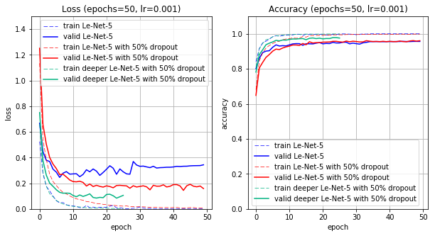
First I tried the standard Le-Net-5 model (see LeNet()function) with the pre-processed grayscale images. The model achieved a good validation set accuracy (94.7% accuracy) but does not generalizes well on the test set (93.3% accuracy) and the five new traffic sign images (80.0% accuracy).

In order to improve the generalization of the model I introduced 50% dropout units in each fully connected layer (see LeNetDropout()function). These units reduced the overfitting of the model. The dropout units increased the test set accuracy by +1.5% and the accuracy on the five new traffic sign images by +20%. Nevertheless, the +20% is not really appreciable because the softmax probability of the 60 km/h electronic speed limit is just at 0.38469. The model is still unsure.

In my final model I increased the depth of each convolutional and fully connected layer in order to further reduce the overfitting. By the increased depth, the model is more capable to handle complex structures in the images. These model changes improved the test set accuracy by +2.8%.

Further improvements will be possible by more complex models. Nevertheless, the training of these models will need a GPU. I trained my model on my local MacBookPro from 2010 (i5 2.53 GHz, 8 GB RAM) on just a CPU which takes roughly 45-60 minutes.

Model Results:

Model	Le-Net-5	Le-Net-5 with Dropout	Deeper Le-Net-5 with Dropout
epochs till stagnation	17	50	25
training set accuracy	99.9%	99.8%	99.9%
validation set accuracy	94.7%	95.5%	97.8%
test set accuracy	93.3%	94.8%	96.1%
5 new signs accuracy	80.0%	100.0%	80.0%

The diagrams below gives an overview about the loss and accuracy over the epochs for the standard Le-Net-5 (blue lines), the Le-Net-5 with two 50% dropout units (red lines) and the deep Le-Net-5 with two 50% dropout units (green lines).

5. Test a Model on New Images

Here are five German traffic signs that I found on the web (extracted from goolge street view). The first row shows the original RGB image, the second row the pre-processed images.

The first image might be difficult to classify because it shows an electronic sign on a German motorway. It looks like an inverted image (white characters and black background). The keep right and yield signs are slightly rotated and tilted which might lead to classification issues.

5.1 Model Predictions on new Images

The code for making predictions on my final model is located in the cell 15 of the IPython notebook.

Here are the results of the prediction:

Image	Prediction	Probability
03-Speed limit (60km/h)	14-Stop	99.82%
01-Speed limit (30km/h)	01-Speed limit (30km/h)	100.00%
03-Speed limit (60km/h)	03-Speed limit (60km/h)	100.00%
38-Keep right	38-Keep right	99.84%
13-Yield	13-Yield	100.00%

The model was able to correctly guess 4 of the 5 traffic signs, which gives an accuracy of 80.0%. The first 60 km/h speed limit sign is hard to predict, because it is not part of the training set. The colors are inverted (black sign background and the white characters).

5.2 Top 5 Softmax Probabilities

The following bar charts give an overview about the top 5 softmax values for each traffic sign prediction.

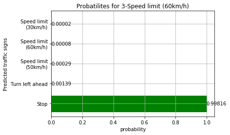
Sign: "Speed limit 60 km/h electronic"

For the first image, the model is wrong and predicted the 60 km/h speed limit sign as stop sign (probability of 0.99816). The top five soft max probabilities were

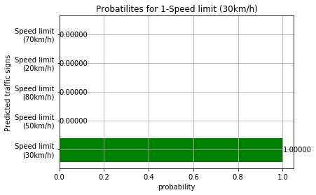
Sign: "Speed limit 30 km/h"

For the second image, the model is relatively sure that this is a 30 km/h speed limit sign (probability of 1.0). The top five soft max probabilities were

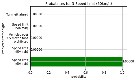
Sign: "Speed limit 60 km/h"

For the third image, the model is absolutely sure that this is a 60 km/h speed limit sign (probability of 1.0). The top five soft max probabilities were

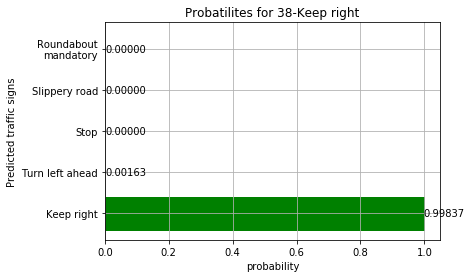
Sign: "Keep right"

For the fourth image, the model is relatively sure that this is a keep right sign (probability of 0.99837). The top five soft max probabilities were

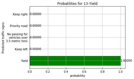
Sign: "Yield"

For the fifth image, the model is absolutely sure that this is a yield sign (probability of 1.0). The top five soft max probabilities were

5.3 Precision, Recall and f1-Score

Precision

The precision is also known as PPV (positive predictive value) and answers the question "What proportion of the instances classified as X is actually an X?"

precision = TP / (TP + FP)

Recall

recall = TP / (TP + FN)

The recall is also known as TPR (true positive rate) and answers the question "What proportion of the real X was actually classified as X?"

f1-Score

The f1-score describes the relationship between the precision and the recall value. 1.0 means best case.

f-score = 2 precision recall / (precision + recall)

The table below shows the precision, the recall and the f1-Score for all signs in the test set.

ID	Signname	Precision	Recall	F-Score	Support
0	Speed limit (20km/h)	98.36 %	100.00 %	0.99	60
1	Speed limit (30km/h)	98.88 %	97.78 %	0.98	720
2	Speed limit (50km/h)	96.62 %	99.20 %	0.98	750
3	Speed limit (60km/h)	97.43 %	92.67 %	0.95	450
4	Speed limit (70km/h)	99.54 %	98.33 %	0.99	660
5	Speed limit (80km/h)	89.31 %	96.83 %	0.93	630
6	End of speed limit (80km/h)	96.67 %	96.67 %	0.97	150
7	Speed limit (100km/h)	95.18 %	96.44 %	0.96	450
8	Speed limit (120km/h)	97.73 %	95.56 %	0.97	450
9	No passing	98.56 %	99.79 %	0.99	480
10	No passing for vehicles over 3.5 metric tons	99.23 %	97.88 %	0.99	660
11	Right-of-way at the next intersection	91.14 %	95.48 %	0.93	420
12	Priority road	99.71 %	98.26 %	0.99	690
13	Yield	99.58 %	99.58 %	1.00	720
14	Stop	98.49 %	96.67 %	0.98	270
15	No vehicles	97.65 %	99.05 %	0.98	210
16	Vehicles over 3.5 metric tons prohibited	100.00 %	99.33 %	1.00	150
17	No entry	99.72 %	97.78 %	0.99	360
18	General caution	97.69 %	86.67 %	0.92	390
19	Dangerous curve to the left	77.92 %	100.00 %	0.88	60
20	Dangerous curve to the right	90.70 %	86.67 %	0.89	90
21	Double curve	94.92 %	62.22 %	0.75	90
22	Bumpy road	99.03 %	85.00 %	0.91	120
23	Slippery road	82.78 %	99.33 %	0.90	150
24	Road narrows on the right	85.42 %	91.11 %	0.88	90
25	Road work	96.11 %	97.92 %	0.97	480
26	Traffic signals	82.22 %	82.22 %	0.82	180
27	Pedestrians	67.19 %	71.67 %	0.69	60
28	Children crossing	94.87 %	98.67 %	0.97	150
29	Bicycles crossing	94.68 %	98.89 %	0.97	90
30	Beware of ice/snow	91.94 %	76.00 %	0.83	150
31	Wild animals crossing	94.70 %	99.26 %	0.97	270
32	End of all speed and passing limits	93.65 %	98.33 %	0.96	60
33	Turn right ahead	95.00 %	99.52 %	0.97	210
34	Turn left ahead	86.23 %	99.17 %	0.92	120
35	Ahead only	98.71 %	98.46 %	0.99	390
36	Go straight or right	97.54 %	99.17 %	0.98	120
37	Go straight or left	100.00 %	98.33 %	0.99	60
38	Keep right	98.11 %	97.97 %	0.98	690
39	Keep left	98.81 %	92.22 %	0.95	90
40	Roundabout mandatory	94.59 %	77.78 %	0.85	90
41	End of no passing	80.00 %	93.33 %	0.86	60
42	End of no passing by vehicles over 3.5 metric tons	94.74 %	80.00 %	0.87	90

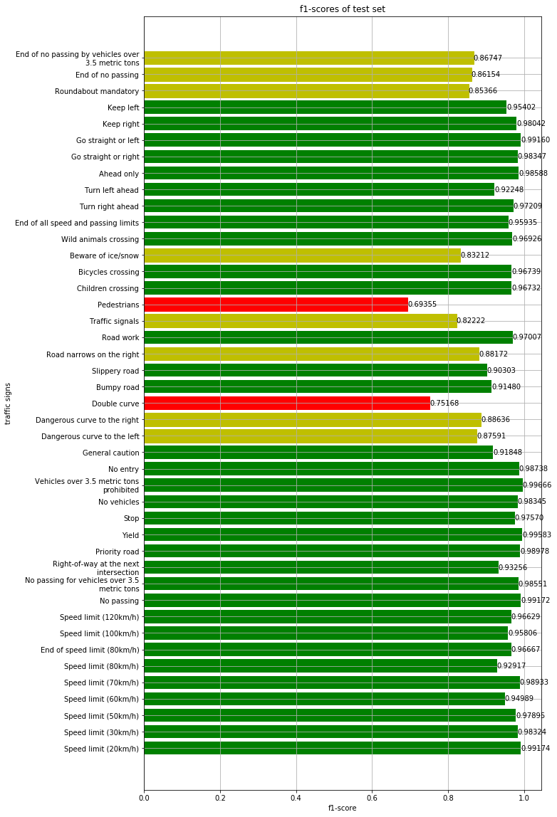
The bar chart summarizes the f1-score over all traffic sign classes. Green bars show classes with a f1-score >0.9 which means a good recall and precision value, yellow bars with a f1-score <=0.9 and red bars with a f1-score <=0.8. The prediction performance of the yellow and red traffic sign classes are not sufficient.

If we compare the yellow and red traffic sign classes with the table above, we can see that these are almost the classes with a low number of training samples. One solution would be to add new sample by augmenting the training data set. This can be done e.g by rotation, zoom and flips.

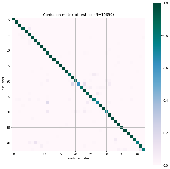
The normalized confusion matrix summarizes the table above. The x-axis indicates the predicted signs by the model and y-axis the real sign (ground truth). The diagonal line describes the points where the IPython sign is equal to the ground truth data. All other areas are false positives.

6. Visualization of the CNN Layers

The following list describes the features maps of the layer 1 activation relu. The activation unit is calculated for the keep right traffic sign.

Feature Map 0 seems to look for round shapes and the arrow line
Feature Map 13 seems to look for round shapes with an right arrow head
Feature Map 2, 7, 11 and 14 seem to look for round shapes with more "clutter/noise" in the background

CNN Layer 1

SvenMuc/CarND-TrafficSignClassifier-P2