
The goal of this project is to develop a pipeline which is capable to detected and track vehicles. The following chapters give a short insight into the feature extraction methods, the classifier, the vehicle detection and tracking mechanisms. Finally the achieved results are discussed an demonstrated in a short video.
The goals / steps of this project are the following:
- Perform a Histogram of Oriented Gradients (HOG) feature extraction on a labeled training set of images and train a classifier Linear SVM classifier
- Optionally, you can also apply a color transform and append binned color features, as well as histograms of color, to your HOG feature vector.
- Implement a sliding-window technique and use your trained classifier to search for vehicles in images.
- Run your pipeline on a video stream (start with the test_video.mp4 and later implement on full project_video.mp4) and create a heat map of recurring detections frame by frame to reject outliers and follow detected vehicles.
- Estimate a bounding box for vehicles detected.
The following list gives a short overview about all relevant files and its purpose.
- VehicleClassifier.py classifies bounding boxes as vehicle or non-vehicle. Furthermore it provides methods to train, save and load the model.
- model.pkl trained classifier model. The pickled file includes the trained model (classifier) and the applied scaler required to normalize the samples (bounding boxes).
- CoreImageProcessing.py provides basic (core) image processing algorithms like spatial binning, color histograms and HOG feature extraction. The same class has been used for the Advanced Lane Finding project. Therefore, the class includes a couple of functions like gradient, magnitude methods which are not used for this project.
- VehicleDetection.py detects and tracks vehicles in an RGB image.
The vehicle classifier classifies bounding boxes as "vehicle" or "non-vehicle". I chose a linear support vector classification from the scikit-learn library (LinearSVC). The classifier has been fitted with a combination three feature sets. The spatially binned, the color channel histograms and the histogram of oriented gradients (HOG) feature sets. The full code can be found in the VehicleClassifier.py file.
To train the classifier the following console parameters have to be used. -t specifies the path to the training examples. -s stores the trained model to the specified pickled file.
python VehicleClassifier.py -t ./train_data -s model.pkl
To use the trained classifier the following lines of code are required. The first line creates an instance of the VehicleClassifier() which loads the trained pickled model. The second line extracts the feature set from a given RGB image, resp. a bounding box and the last line predicts whether the bounding box is of type "vehicle" or "non-vehicle". Additionally to the predicted class the method returns the confidence score which is the signed distance of that sample to the hyperplane.
classifier = VehicleClassifier('model.pkl')
features = classifier.extract_features(rgb_image)
predicted_class, confidence = classifier.predict(features)For the training of the classifier I used the already labeled GTI and the KITTI dataset. My dataset consists of 17760 samples which are labeled as "vehicle" and "non-vehicle". The two classes are well balanced as shown in the table below.
| Label | Samples | Percentage | Udacity Download Link |
|---|---|---|---|
| vehicles | 8792 | 49,5 % | DB "vehicles" |
| non-vehicles | 8968 | 50,5 % | DB "non-vehicles" |
For the first feature set I use three spatially binned color channels. The method bin_spatial(self, img, size=(32, 32)) first resizes the img (bounding box) to the size and concatenates the raw pixel values to an 1D feature vector.
The pictures below shows typical feature vectors of the class "vehicle" and the "non-vehicle" in different color spaces. The images are scaled down from 64x64 to 32x32 pixels which leads to an feature vector length of 32 * 32 * 3 channels = 3072. The difference between a "vehicle" and a "non-vehicle" feature set is clearly visible in the diagrams.
Class: "Vehicle"

Class: "Non-Vehicle"

In order to find the best hyper-parameters for the spatially binned feature set, I trained a LinearSVC and varied the color space and image size. In total I used 4000 samples which has been split into a training dataset (80%) and a test dataset (20%).
Tested Hyper-Parameters:
- color space (RGB, LUV, HLS, YUV, YCrCb)
- image size (8x8, 16x16, 32x32)
The diagram below shows all accuracy results on the test dataset. One interesting characteristics is that there seems to be no correlation between the accuracy and the applied image size. This strongly depends on the applied color space. E.g. the 16x16 image sizes in the RGB, LUV, HLS and YUV color space shows a slightly lower accuracy score than the lower image size with 8x8 pixels.
Best accuracy scores (≥90 %) have been achieved with an image size of 32x32 in the RGB, LUV and YCrCb color channels.

For the second feature set I use color histograms of all 3 color channels of an image. The method color_histogram(self, image, nb_bins=32, features_vector_only=True) splits the image into three color channels and calculates the histogram for each of these channels separately. Afterwards it concatenates the individual bin values into a 1D feature vector.
The charts below show typical results of the class "vehicle" and "non-vehicle". In the middle you can see the histograms with a bin size of 32 for the red, green and blue color channels. On the right the 1D feature vector is depicted. A histogram bin size of 32 leads to a feature vector length of 32 bin * 3 channels = 96.
Class: "Vehicle"

Class: "Non-Vehicle"

In order to find the best hyper-parameters for the color histogram I applied the same method as described in chapter 3.3 Spatially Binned Features above. The diagram below shows all accuracies on the test dataset.
Tested Hyper-Parameters:
- color space (RGB, LUV, HLS, YUV, YCrCb)
- number of histogram bins (8, 16, 32, 64, 128)
Best accuracies (≥92 %) have been achieved for LUV with 32 bins, HLS with 64 bins and YCrCb with 64 bins.

The last feature set is based on the histogram of oriented gradients (HOG) method. The method hog_features(self, img, channel, orient, pix_per_cell, cell_per_block, vis=False, feature_vec=True) calculates the HOG features on the given img for the specified color channel and returns a 1D feature vector. For further details about the HOG calculation have a look to the paper Histograms of Oriented Gradients for Human Detection, Navneet Dalal and Bill Triggs.
The charts below show typical results of the class "vehicle" and "non-vehicle". In the top row you can see the YCrCb image followed by the Y, Cr and Cb channels. The second row depicts the corresponding HOG images (orientations) and the last row the 1D feature vectors.
The length of the shown HOG feature vector can be calculated as followed:
- number of block positions = (64 pixel / 8 cells per block - 1)^2 = 49
- number of cells per block = 2 * 2 = 4
- number of orientations = 9
- Total length single channel = 49 * 4 * 9 = 1764
- Total length all channels = 1764 * 3 = 5292
This simple calculation shows, that the feature vector can get easily quite long which is extremely critical regarding the computing time. In oder to realize an system which is capable to run online in a vehicle the parameters have to chosen carefully.
Class: "Vehicle"

Class: "Non-Vehicle"

In order to find the best hyper-parameters for the HOG feature set, I applied a slightly changed method as described in chapter 3.3 Spatially Binned Features above. I limited the number of orientations to 8, because higher numbers led to critical computing times. Furthermore, several test runs showed that the number of pixels per cell of 8 and the number of cells per block of 2 are suitable for this type of problem. Afterwards, I tested all variants of color spaces and usage of color channels. The diagram below shows all accuracies on the test dataset.
Tested Hyper-Parameters:
- color space (RGB, LUV, HLS, YUV, YCrCb)
- color channels (all, 0, 1, 2)
Best accuracies (≥97 %) have been achieved for the HLS, the YUV and the YCrCb color space in combination with all color channels.

After tuning of the individual methods like spatial binning, color histograms and HOG features I combined the best three feature sets and fine tuned its hyper-parameters in order to find an optimum between the accuracy and the computing time. The parameter setup in the YCrCb color space with 16 orientations in the HOG method achieved the best accuracy of 99,5 %. But due to the high computing time I chose the second best results with 99,25 % which almost needs 1/4 less computing time. The whole feature extraction pipeline has been implemented in the method extract_features(self, img_rgb).

Final Hyper-Parameters
   spatial_size = (32, 32)                # size of spatially binned image
   hist_nb_bins = 64                      # number if histogram bins
   hog_orient = 10                        # number of HOG orientations
   hog_pix_per_cell = 8                   # number of pixels per cell
   hog_cell_per_block = 2                 # number of cells per block
hog_channel = 'ALL' # number of HOG channels, can be 0, 1, 2, or 'ALL'First I tried the simple sliding window approach which turned out to be extremely slow, especially when you apply multi-scaled windows. Therefore, I decided to implement the "HOG sub-sampling method" (see find_vehicles(self, img_rgb, y_start, y_stop, scale, cells_per_step)). The basic idea of this method is that you calculate the computational intensive HOG function once on a cropped and scaled down image. The ROI is defined by y_start to y_stop and the scaling factor by scale. Afterwards, the scaled image is sub-sampled to calculate the other feature sets like spatial binning and color histogram.
The image below exemplary shows the steps for the HOG feature calculation.

The source code can be found in find_vehicles(self, img_rgb, y_start, y_stop, scale, cells_per_step):
- crop the input RGB image
img_rgbto the defined ROI[y_start, y_stop] - convert the cropped image into YCrCb color space
- calculate the HOG features of all 3 YCrCb channels in the scaled image
- apply the sliding window method and calculate the spatial binned and color histogram feature set for each window
- concatenate all feature sets to a 1D feature vector (
test_features) - predict every window whether it is of the class "vehicle" or "non-vehicle" (
test_predictionandtest_confidence) - append the bounding box and confidence score for all windows classified as "vehicle" and a confidence ≥0.5 to the vehicle candidate lists (
bboxes,confidence) - finally generate a heatmap of bounding boxes in the
bboxesarray
The heart of the vehicle detection pipeline is located in the detect_vehicles(self, img_rgb) method. This method consist of the following processing steps.
First I search in three regions (near, mid and far) for vehicle candidates. This step is required to detect vehicles at different distances. Therefore, I call the find_vehicles() method on the different ranges (y_start and y_stop), different scale factors and different cells_per_step configurations. The code snippet below shows the applied values.
conf_threshold = 0.5                   # min confidence threshold for vehicle candidates
roi_far_range = [400, 500, 1.1, 1]     # [ROI min y, ROI max y, scale factor, cells per step]
roi_mid_range = [400, 600, 1.5, 2]     # [ROI min y, ROI max y, scale factor, cells per step]
roi_near_range = [400, 656, 2.6, 2]    # [ROI min y, ROI max y, scale factor, cells per step]
After this processing step I receive three different heatmaps and bounding box lists for the different ranges (Bounding Boxes: near range = violet, mid range = cyan, far range = yellow). The heatmaps are finnaly summed up to one heatmap as shown in the bottom right chart.

In order to stabilize the vehicle detection and reduce false positives, I use a history of heatmaps over the last 8 frames. The older the heatmap, the less important it is for the actual frame. Therefore, the heatmap history is cumulated in one heatmap with different weight factors. Afterwards, I applied a simple threshold function in order to remove the clutter which are candidates for false positives.
As next step we have to identify the vehicle bounding box by analyzing the thresholded heatmap. I used the scipy.ndimage.measurements.label() method for this step because it returns a labeled array indicating regions belonging together. I assumed that each of this region corresponds to a vehicle. The image sequence below summarized all processing steps.
From left to right, you can see the vehicle candidates of the actual frame, followed by the cumulated weighted history heatmap, the thresholded heatmap and finally the labeled regions. In the last step, the labeled data are converted the vehicle bounding boxes and drawn as green boxes in the first image.

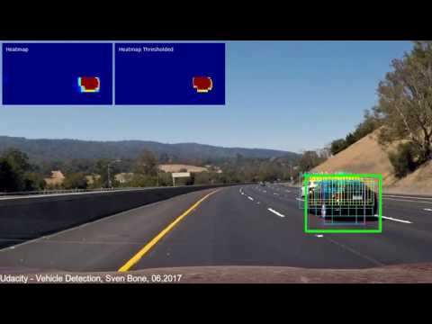
The image below shows the detect_vehicles() input image with all activated debug overlays. In the top left the cumulated weighted history heatmap is displayed, followed by the thresholded heatmap. The vehicle candidates (intermediate results of the find_vehicles() method) are depicted depending on the search range in yellow (FAR), cyan (MID) or violet (NEAR). Each bounding box indicates its confidence score at the top left corner. Finally confirmed vehicle detections are represented by a green bounding box.

Video on GitHub
YouTube Video
This project applies kind of old fashioned methods. However it's was extremely valuable to go through all these processing steps like HOG, spatial binning, color histogram, heatmaps, etc. in order to get a better feeling how difficult and time consuming the manual parameter tuning process could be. Furthermore, this experience helps to better judge the pros and cons of newer or alternatives concepts.
My pipeline works well on the used video clip but is far away from a function that could be used in a real product. The pipeline e.g has problems when two vehicles in the image are located too close to each other. In that case its bounding boxes are merged together. Possible solutions would be to classify the color of each vehicle or to estimate its position in world coordinates and compare its relative speeds to better distinguish them. This would require the setup e.g. a kalman filter to track and to estimate the object's movements.
Furthermore the scipy.ndimage.measurements.label() method is not a robust solution. Sometimes it splits a vehicle bounding box into two separate boxes. To further improve the position accuracy better vehicle segmentation algorithms have to be implemented. And finally the sliding window method is extremely computational intensive. Special hardware like FPGAs could solve this.
Alternative concepts are based on Deep Neural Networks (DNNs). The paper "Image-based Vehicle Analysis using Deep Neural Network: A Systematic Study" gives a short overview about state of the art networks. The big advantage of this approach is that the time consuming feature set generation and the faulty parameter tuning gets obsolete. But this concept has also some drawbacks. You shift the time consuming efforts to the generation of a highly accurate and well labeled dataset.