This project aims to predict the presence of cancer based on gene expression data from the Gene Expression Omnibus (GEO) database. RNA sequencing data from cancer and non-cancer samples will be analyzed to identify differences in expression profiles. By focusing on a subset of key genes related to cancer development, the project will explore how gene expression patterns differ between cancerous and normal tissues, and whether these patterns can be used to predict the likelihood of cancer.
Proteins are essential for the fulfillment of critical processes throughout the body. The instructions for making these proteins are encoded in our genes, and proteins are produced through the expression of these genes. When there is a malfunction in this protein-making process, it can lead to diseases such as cancer.
Abnormal gene expression is often a sign of cancer and has been used in personalized medicine to identify targets for precision treatments. The data used to detect abnormal gene expression comes from RNA sequencing (RNA-seq), which measures the frequency of gene expression in cells. RNA-seq provides information about which genes are being expressed and at what levels, based on the presence of RNA. The actual values in RNA-seq data represent counts of RNA fragments that have been mapped (or connected) to specific genes, reflecting how actively a gene is being expressed in a given sample.
The main goal is to successfully predict cancer based on the RNA expression levels of a few genes of interest. These genes will be selected based on their known association with cancer-related pathways or their differential expression between cancer and normal tissue samples. The project will -
- Identify key genes with significant expression changes between cancerous and healthy tissues.
- Build predictive models to classify samples as cancerous or non-cancerous based on RNA expression levels.
Data will be sourced from the publicly available Gene Expression Omnibus (GEO) repository. Specific datasets containing RNA sequencing data from cancer patients and healthy controls will be identified and downloaded. These datasets typically include thousands of genes, but the focus will be on a subset of genes that are strongly linked to cancer progression, based on existing literature or feature selection techniques. Steps to collect data -
- Identify suitable GEO datasets containing both cancer and healthy control samples.
- Filter the data to focus on a few key genes (approximately 10-20 genes) related to cancer biology.
- Preprocess the data to remove noise and normalize gene expression values for further analysis.
Our selected dataset, sourced from the Gene Expression Omnibus (GEO) and hosted on Kaggle, contains RNA sequencing data from Tumor-Educated Platelets (TEPs). TEPs are known to reflect tumor presence in the body, as their RNA profiles change in response to signals released by tumors into the bloodstream. Leveraging TEPs for cancer diagnostics and treatment is an emerging area of research, making this dataset highly relevant for modeling applications.
The dataset comprises 283 blood platelet samples, including 55 from healthy individuals, representing the cancer types of non-small cell lung, colorectal, pancreatic, and breast cancer, along with glioblastoma and hepatobiliary carcinomas. Each sample provides expression levels for 57,736 genes. Additionally, the dataset includes intron-spanning data, which offers insights into how tumors may influence RNA splicing—the process of removing non-coding regions from RNA.
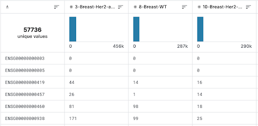
Figure 1. Snippet of Uncleaned Dataset from Kaggle
The initial step in data cleaning was to remove redundant information that would not contribute to predicting cancer through modeling. For example, a column identifying the species from which the sample originated was dropped, as all samples were from humans.
Next, the cancer type classification for each sample was one-hot encoded to make it usable in modeling techniques. The dataset format was then converted from wide (with each sample as a column and each row showing the expression level of a specific gene) to long format, where the sample identifiers and gene expression levels are organized into dedicated columns. Finally, the cancer type labels were mapped back to ensure the one-hot encoded cancer type columns followed the gene_ID, sample, and FPKM (expression level) columns. The healthy control samples were also included in this format, with their cancer type encoded as Cancer_Type_HC (healthy control).

Figure 2. Snippet of Cleaned Dataset Columns
To visualize the differences in gene expression between cancerous and normal tissues, the following techniques will be used -
- Box plots to compare the distribution of expression levels for each selected gene between cancer and non-cancer groups.
- Heatmaps to display the relative expression levels of multiple genes across different samples, highlighting patterns of differential expression.
- t-SNE or PCA plots to project high-dimensional gene expression data into a lower-dimensional space, providing visual insights into how cancerous and non-cancerous samples cluster based on their gene expression profiles.
- Interactive scatter plots to visualize the relationship between two or more gene expression levels and how these relate to cancer classification.
To better understand the dataset, a series of visualizations were created to highlight gene expression patterns and their potential implications for cancer diagnostics.
In Figure 3, we observe that the differential expression of genes between breast cancer and normal samples varies significantly. Some genes, such as 166170, show substantial expression differences, suggesting their potential as strong predictors. This gene also appears to be differentially expressed across all cancer samples (Figure 4), indicating its association with cancer in general. According to The Human Protein Atlas, 166170 has low cancer specificity, making it useful for distinguishing between cancerous and non-cancerous samples, though less effective for identifying specific cancer types (B2M).
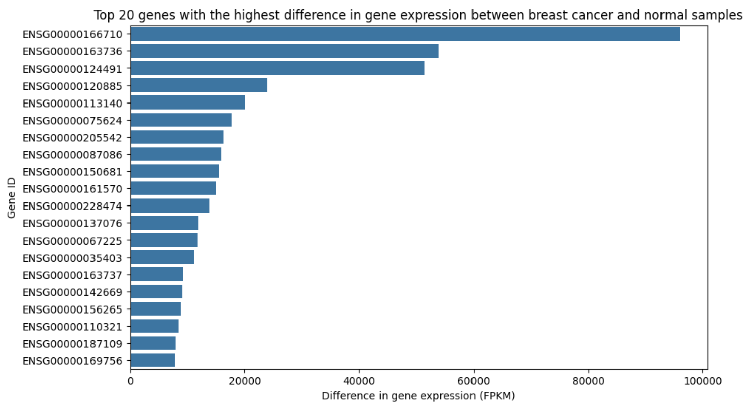
Figure 3. Comparison of Top 20 Differentially Expressed Genes in Breast Cancer and Healthy Samples
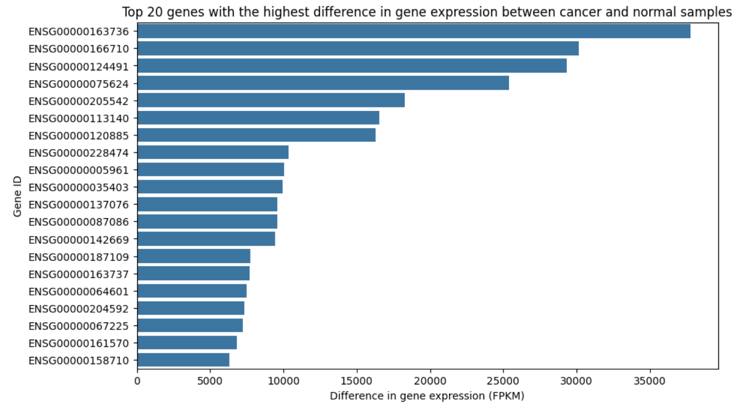
Figure 4. Comparison of Top 20 Differentially Expressed Genes in Cancer and Healthy Samples
Next, Figure 5 compares the mean values of the top 20 differentially expressed genes between cancerous and healthy samples. While it overlaps somewhat with the information in Figure 4, this heatmap adds context by displaying mean FPKM values, highlighting the origins of these differences. For example, gene 205542 has a notably higher mean FPKM compared to other genes with similar differential expressions.
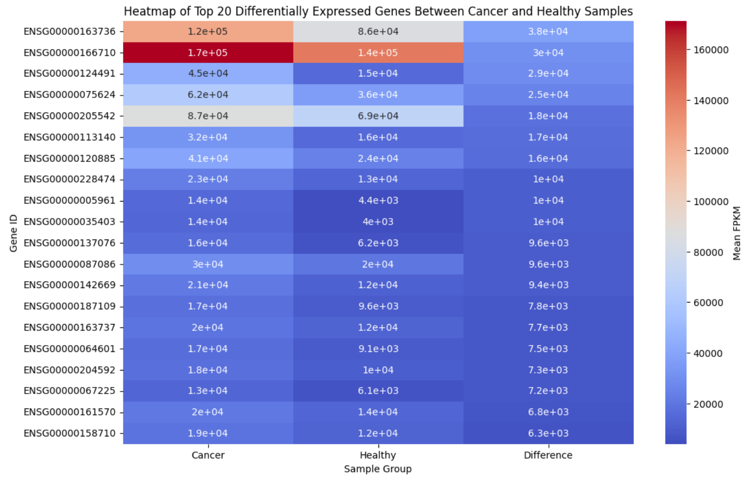
Figure 5. Heatmap Comparison of Top 20 Differentially Expressed Genes Between Cancerous and Healthy Samples
Using a violin plot (Figure 6) helped elucidate the distribution of log-transformed FPKM values across the top 20 differentially expressed genes. A consistent pattern from this chart is that, on average, non-cancerous samples exhibit lower mean FPKM values than cancerous samples. Additionally, certain genes, such as 149311, display a broader distribution or multiple peaks in the non-cancerous samples, a characteristic that could enhance model performance.
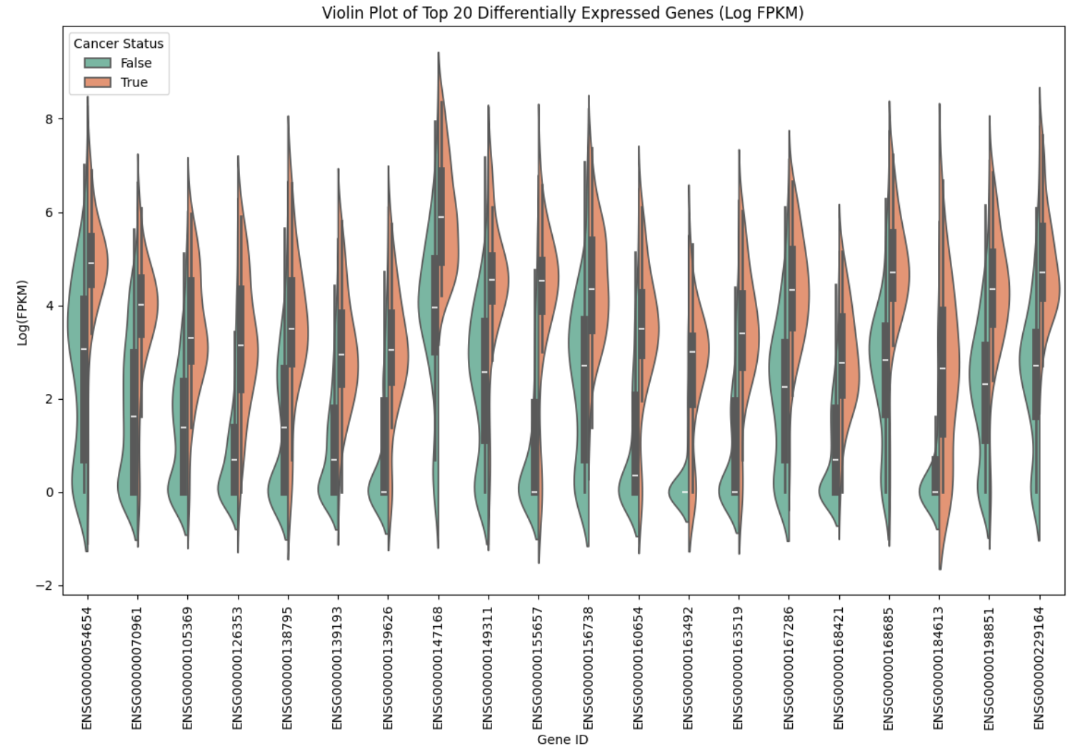
Figure 6. Violin Plot of Top 20 Differentially Expressed Genes (Log FPKM)
During this visualization process, it became evident that gene expression levels required normalization due to wide variability in values. Normalizing expression differences ensured that patterns reflected biological relevance rather than technical variability. Figure 7 shows the top 20 differentially expressed genes after normalization, illustrating how this step helped clarify the data for further analysis.
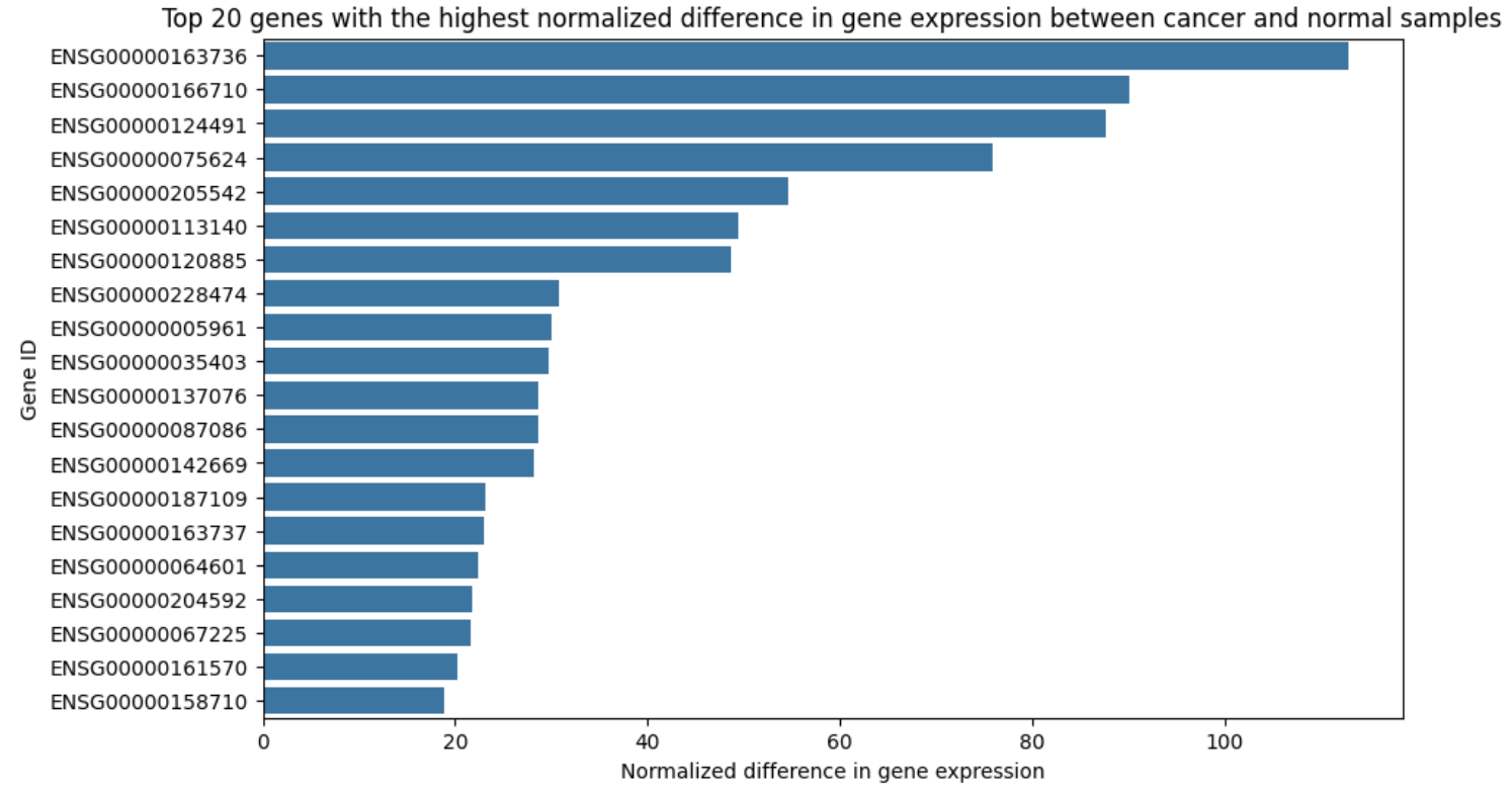
Figure 7. Comparison of Top 20 Normalized Differentially Expressed Genes between Cancerous and Healthy Samples.
Following this, Figure 8 provides insight into how FPKM values vary within each of the top 20 differentially expressed genes. Some genes show much wider distributions of expression levels than others. For instance, gene 187109, which has low cancer specificity, displays a tight distribution compared to gene 163736 (NAP1L1; PPBP), which is specifically associated with colorectal cancer. These distribution characteristics are essential considerations when building a model, as they may impact predictive accuracy.
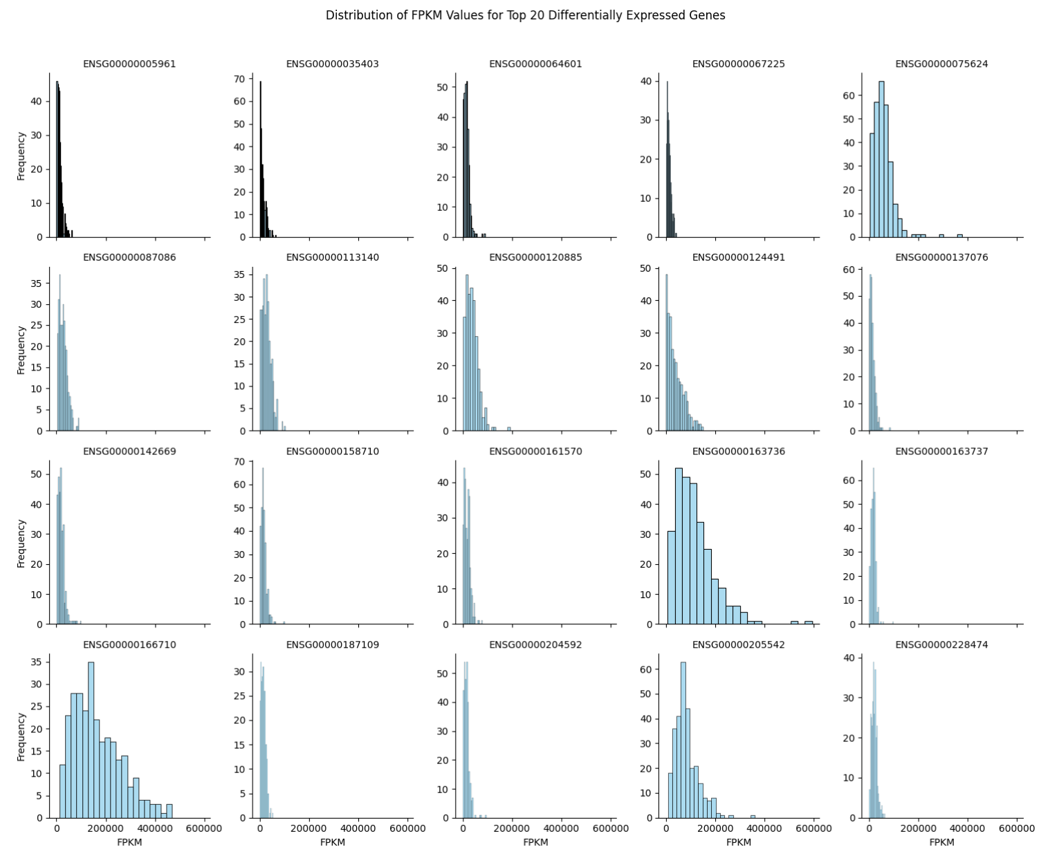
Figure 8. Facet Grid of FPKM Distribution of Top 20 Differentially Expressed Genes
To model the data, several machine learning methods will be explored -
- Logistic Regression - A simple linear model will be used as a baseline to assess how well gene expression levels can predict cancer.
- Decision Trees or Random Forests - Non-linear models will be used to capture complex interactions between gene expression levels and cancer classification.
- Support Vector Machines (SVM) - SVM is a method to classify samples based on their gene expression profiles, particularly useful for binary classification tasks like cancer detection.
- XGBoost or Gradient Boosting Machines - This are tree-based ensemble methods that could potentially outperform simpler models.
- Deep Learning (optional) - If needed, a neural network might be employed to identify complex patterns in gene expression data.
The choice of the model will depend on the performance in predicting cancer from the training data.
The test plan involves splitting the data into training and testing sets -
- 80-20 split - 80% of the dataset will be used for training the model, and the remaining 20% will be withheld for testing the model’s performance.
- Cross-validation - To ensure the robustness of the model, k-fold cross-validation (with k=5 or 10) will be employed during training.
- Performance Metrics - The model will be evaluated based on accuracy, precision, recall and F1-score, as cancer detection often involves trade-offs between false positives and false negatives.
- Test on external data - If possible, after building the model on one dataset, it will be tested on a different GEO dataset to check the generalization of the model.
Before modeling, the data was standardized and split into training and testing sets, with 80% allocated for training and 20% for testing.
The top 20 differentially expressed genes were used as input features for a Random Forest model. Using RandomizedSearchCV, the optimal hyperparameters were identified by testing 20 random combinations with 5-fold cross-validation. Random states were set for reproducibility. The best model configuration included no bootstrapping, balanced class weights, a maximum depth of 30 for each tree, a minimum of 2 samples per leaf node, and 200 trees in the forest. This model achieved an accuracy of 0.96. However, a key limitation is its recall score of 0.33, indicating poor performance in classifying breast cancer samples. Although this is an improvement over initial tests that couldn’t predict breast cancer at all, expanding the feature set will likely be necessary to boost model performance further.
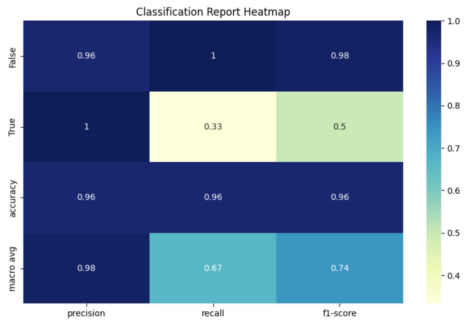
Figure 9. Random Forest Classification Report Heatmap - Top 20 Differentially Expressed Genes Between Breast Cancer and Healthy Samples
XGBoost was also used to classify samples by specific cancer type, with cancer types encoded as numerical values from 0 to 11 (Figure 10). Interestingly, this model performed well in identifying healthy control samples but struggled with the cancerous samples (Figure 11). This outcome may be due to the distribution of the dataset: while there are only 55 healthy samples, the remaining samples are divided among 11 different cancer types, giving healthy samples a relatively higher representation. To improve the classification of specific cancer types, we could explore assigning weights to genes known to be associated with certain cancers, as highlighted in earlier visualizations.
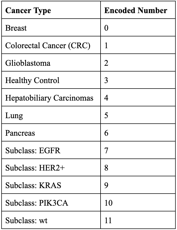
Figure 10. Numerically Encoded Cancer Types
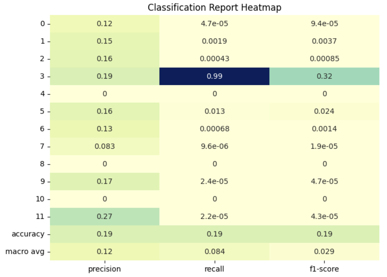
Figure 11. XGBoost Classification Report Heatmap - All Cancer Types
The most recent model we fitted was logistic regression. Before fitting this model, we used Principal Component Analysis (PCA) to reduce the dimensionality of the data. The logistic regression model was then trained on the reduced dataset, yielding results similar to previous models (Figure 12). While the model performed reasonably well at predicting healthy samples, it struggled to accurately classify the other cancer types.
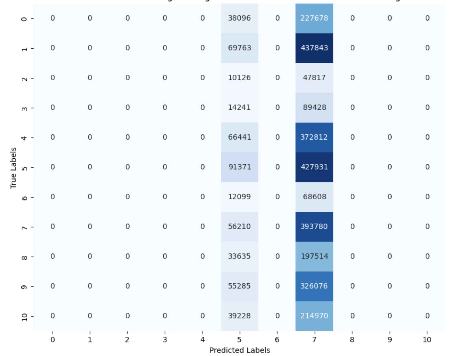
Figure 12. Logistic Regression Classification Report Heatmap - PCA Reduced Data
As we move into the next phases of the project, we aim to streamline the insights gained from our initial modeling attempts. One key area for improvement is addressing the oversampling of healthy controls, which appears necessary to enhance model performance. So far, the Random Forest model has yielded the best results, though this was only tested on distinguishing breast cancer from healthy samples. To improve accuracy across all cancer types in the dataset, we plan to investigate the genes included and assess whether known associations with specific cancer types could inform our model. Additionally, we will explore alternative models, such as Support Vector Machines (SVM) or Deep Learning approaches, which may offer better classification performance than the methods used thus far.
This project will provide insights into how well RNA expression profiles can predict cancer. By focusing on specific genes known to play a role in cancer development, the project will seek to identify patterns in gene expression that can be used as biomarkers for cancer detection. The work will contribute to the understanding of cancer biology and the potential application of machine learning techniques in genomics-based cancer prediction.
Works Cited B2M Protein Expression Summary - The Human Protein Atlas. https://www.proteinatlas.org/ENSG00000166710-B2M. Accessed 3 Nov. 2024. Gene Expression Omnibus (GEO) Dataset: GSE68086. https://www.kaggle.com/datasets/samiraalipour/gene-expression-omnibus-geo-dataset-gse68086. Accessed 3 Nov. 2024. NAP1L1 Protein Expression Summary - The Human Protein Atlas. https://www.proteinatlas.org/ENSG00000187109-NAP1L1. Accessed 3 Nov. 2024. PPBP Protein Expression Summary - The Human Protein Atlas. https://www.proteinatlas.org/ENSG00000163736-PPBP. Accessed 3 Nov. 2024.