

A simple library to build easily interpretable computational constructs similar to Turing machines over graphs, where states can be (but are not limited to) combinations of a graph's (typed) nodes; an example use would be a transparent backend logic which navigates a network of sub-states
pip install Graph_State_Machine
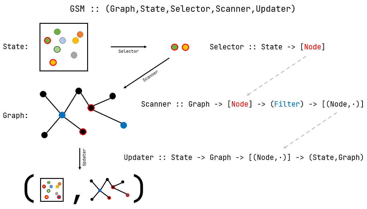
This package implements a computational construct similar to a Turing machine over a graph, where states are typically node combinations (state objects can be arbitrary) and where the arbitrary transition function can update both state and graph. Note that this last arbitrariness makes the system Turing complete since it allows implementing a Turing machine with it (achieved by defining the graph to be a linear array and the state as a tuple of node name and "head" state).
Given a graph with typed nodes and a state object from which a list of nodes can be extracted
(by an optional Selector function), the construct applies two arbitrary functions to perform a step:
Scanner- A generalised neighbourhood function, which scans the graph "around" the state nodes and returns a scored list of nodes for further processing; additional and optional arguments can be included, e.g. to filter by type
Updater- A function to process the scan result and thus update the state and possibly the graph itself
This computational construct is different from a finite state machine on a graph and from a
graph cellular automaton, but it shares some similarities with both in that it generalises some of
their features for the benefit of human ease of design and readability.
For example, a GSM's graph
generalises a finite state machine’s state graph by allowing the combinations of nodes to represent
state, and the scanner function is just a generalisation of a graph cellular automaton’s neighbourhood
function in both domain and codomain.
As previously mentioned, it is closer to a Turing machine on
a graph than either of the above, one whose programming is split between the internal state rules
and the graph topology, thus allowing programs to be simpler and with a more easily readable state.
Said graph topology can be further enriched/simplified by the presence of arbitrary information in the form of node or edge attributes, which can then be used by arbitrary step rules; an example of this are attributes representing necessity and sufficiency of those links.
Besides pure academic exploration of the construct, some uses for it are implementing backend logics which are best represented by graphs (e.g. an "expert system"), or pathing through ontologies by entity proximity or similarity.
(Inspecting the package __init__.py imports is a quick and useful exercise in understanding the overall structure, while the following is a less concise version of the content of types.py)
Formalising the above description using library terminology, the constructor of the main class
(GSM) takes the following arguments:
Graph- A graph object with typed nodes (wrapping a NetworkX graph), with utility methods so that it can be built from shorthand notation (structured edge lists), check its own consistency, self-display and extend itself by joining up with another with common nodes (exact ontology matching)
State- The initial state; the default type is a simple list of nodes (strings), but it can be anything as
long as the used
Scannerfunction is designed to handle it and a function to extract a list of strings from it is provided as the Selector argument Scanner(Graph -> List[Node] -> ... -> List[Tuple[Node, Any]])- A function taking in a list of state nodes to use to determine next-step candidates; arbitrary additional arguments, optional or required, may be present after Graph and List[Node], for example focussing the scan on specific node types; these extra arguments can be passed through the step methods either named (dictionary) or unnamed (list)
Updater(State -> Graph -> ScanResult -> Tuple[State, Graph])- A function taking in the current state and graph along with the result of a node scan and returns the updated state and graph
Selector(State -> List[Node])- A function to extract from the state the list of nodes which should be fed to the Scanner
A simple example of node-list state with non-identity Selector is a GSM which only takes the last
"visited" node into account, and going one step further, an intuitive example of State which is not
a simple node-list is a dictionary of node-lists only some subsets of which are considered for graph
exploration (and others for state updating), e.g. keeping track of which nodes were initial state and
which ones were added by steps.
Simple default constructor functions for this State type are provided:
dict_fields_getter (for selector), which takes in the list of fields to concatenate, and list_in_dict_accumulator (for Updater), which takes in the single field to update.
Since the underlying object is a NetworkX graph, the wide variety of functionality that library provides can easily
be made use of,
but, as previously mentioned, even simply adding arbitrary node and edge attributes can greatly enhance/simplfy a GSM's
processing.
For example, necessity and sufficiency relationships are a reasonable addition to the graph for typical usecases,
therefore support for them is built into the provided Scanner functions, graph creation shorthand and
plotting method(s).
Graphs can be created quickly by letting the Graph class constructor directly parse a specific format of
typed adjacency list, one with Python type signature
Dict[NodeType, Dict[Node, Union[List[Node], Dict[str, List[Union[Node, List[Node]]]]]]]
(Node and NodeType are just convenient aliases for str)
and following this structure:
dict(
    NodeType = dict(
        Node = <NODES TO WHICH THERE IS AN EDGE>,
        ...
    ),
    ...
)
where <NODES TO WHICH THERE IS AN EDGE> can be:
an empty list: no edges to the base node are being declared at this point (but could be declared from the node at the other end)
a list of
Node-s[If the intention is to have necessity and sufficiency relationships] a dictionary of lists of
Node-s, with possible entries:necessary_for: nodes for which the base node is necessary sufficient_for: nodes for which the base node is sufficient are_necessary: nodes which are necessary for the base node are_sufficient: nodes OR LISTS OF NODES which are individually or jointly sufficient for the base node plain: nodes which share and edge with the base node without necessity or sufficiency relationships (at least not declared here)
The structure checks that every node is declared as of some type, and it identifies redundancies and clashes, respectively raising warnings and errors. These checks granted, edges and necessity/sufficiency relationships can be added at either node declaration.
Two convenience functions are provided for writing the inner dictionaries of the typed adjacency list more naturally:
strs_as_keys: given a list ofNode-s (strings), create a dictionary of empty lists with them as keys; for batch declaration of nodes without (for the moment) declared edges. Schematic example:[A, B] -> {A: [], B: []}reverse_adjacencies: given a<NODES TO WHICH THERE IS AN EDGE>, return the reverse-direction<NODES TO WHICH THERE IS AN EDGE>, possibly losing singletons and joint-sufficiency relationships (allow_losing_singletonsandallow_losing_joint_sufficiencyarguments areFalseby default, raising exceptions to prevent losses). This is useful when it is more natural to declare nodes of a specific type as the endpoint of edges from other nodes (perhaps of mixed types); e.g. when the node type in question is semantically a feature or qualifier applicable to more than one kind of entity (like'Data Features'in the exaple below). Schematic example:{A: [B, C], D: []} -> {B: [A], C: [A]}
Use of necessity and sufficiency attributes is on by default in the provided Scanner functions,
and a detailed warning is produced if possibly problematic graph features occur,
but for the sake of user customisation, experimentation and debugging,
support for each can be turned off separately by setting the Scanner-s' check_necessity and/or check_sufficiency
arguments to False (either when constructing the GSM or individually at each GSM.step call).
(The warning will appear if required and contains more details, but the gist of the possible issue is that the presence of neither-necessary-nor-sufficient neighbours of a candidate node in the state does not protect against the absence of sufficient ones).
A small GSM which selects the appropriate R linear regression function and distribution family from labelled data features:
- Define a numerical data-type ontology graph in the typed edge-list shorthand which
Graphaccepts along with ready-made Networkx graphs, making use of two simple notation helper functions - Create a default-settings
GSMwith it and a simple starting state - Ask it to perform steps focussing on the node types of 'Distribution', 'Methodology Function' and 'Family Implementation', which in this context just means finding the most appropriate of each
from Graph_State_Machine import *

_shorthand_graph = {
    'Distribution': {
        'Normal': ['stan_glm', 'glm', 'gaussian'],
        'Binomial': ['stan_glm', 'glm', 'binomial'],
        'Categorical': ['stan_polr', 'polr_tolerant', 'multinom'],
        'Poisson': ['stan_glm', 'glm', 'poisson'],
        'Beta': ['stan_betareg', 'betareg'],
        'Gamma_': ['stan_glm', 'glm', 'Gamma'],
        'Inverse Gaussian': ['stan_glm', 'glm', 'inverse.gaussian']
    },
    'Family Implementation': strs_as_keys(['binomial', 'poisson', 'Gamma', 'gaussian', 'inverse.gaussian']),
    'Methodology Function': strs_as_keys(['glm', 'betareg', 'polr_tolerant', 'multinom', 'stan_glm', 'stan_betareg', 'stan_polr']),
    'Data Feature': reverse_adjacencies({ # Reverse-direction definition here since more readable i.e. defining the contents of the lists
        'Binomial': ['Binary', 'Integer', '[0,1]', 'Boolean'],
        'Poisson': ['Non-Negative', 'Integer', 'Consecutive', 'Counts-Like'],
        'Categorical': ['Factor', 'Consecutive', 'Non-Negative', 'Integer'],
        'Normal': ['Integer', 'Real', '+ and -'],
        'Beta': ['Real', '[0,1]'],
        'Gamma_': ['Non-Negative', 'Integer', 'Real', 'Non-Zero'],
        'Inverse Gaussian': ['Non-Negative', 'Integer', 'Real', 'Non-Zero'],
        'polr_tolerant': ['Consecutive']
    })
}

gsm = GSM(Graph(_shorthand_graph), ['Non-Negative', 'Non-Zero', 'Integer']) # Using default arguments
    # The default node_scanner is by jaccard similarity score, and takes additional arguments to filter candidates
    # and their neighbours by type; only the first one (candidate type list) is used in the examples below

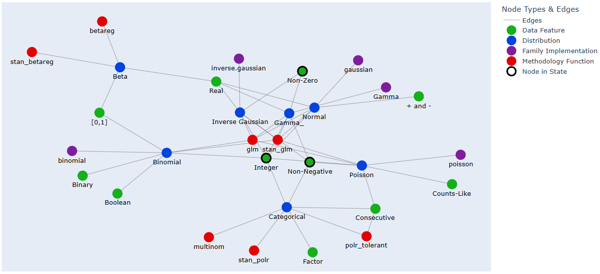
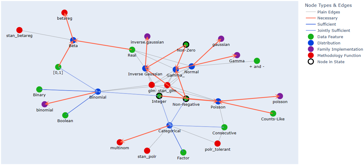
gsm.plot()
# import networkx as nx
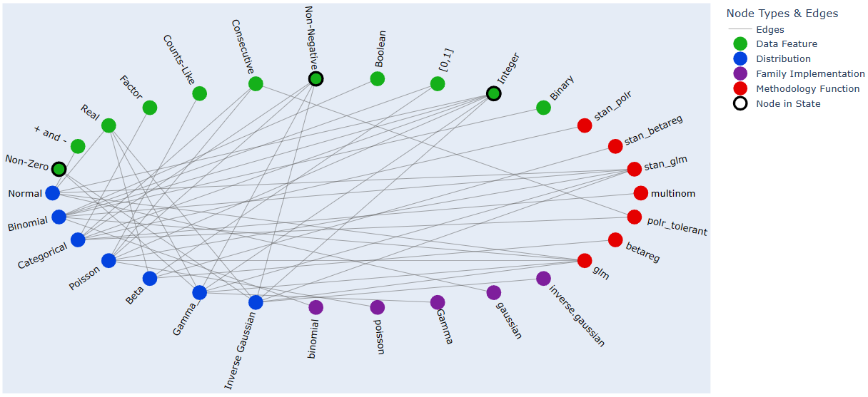
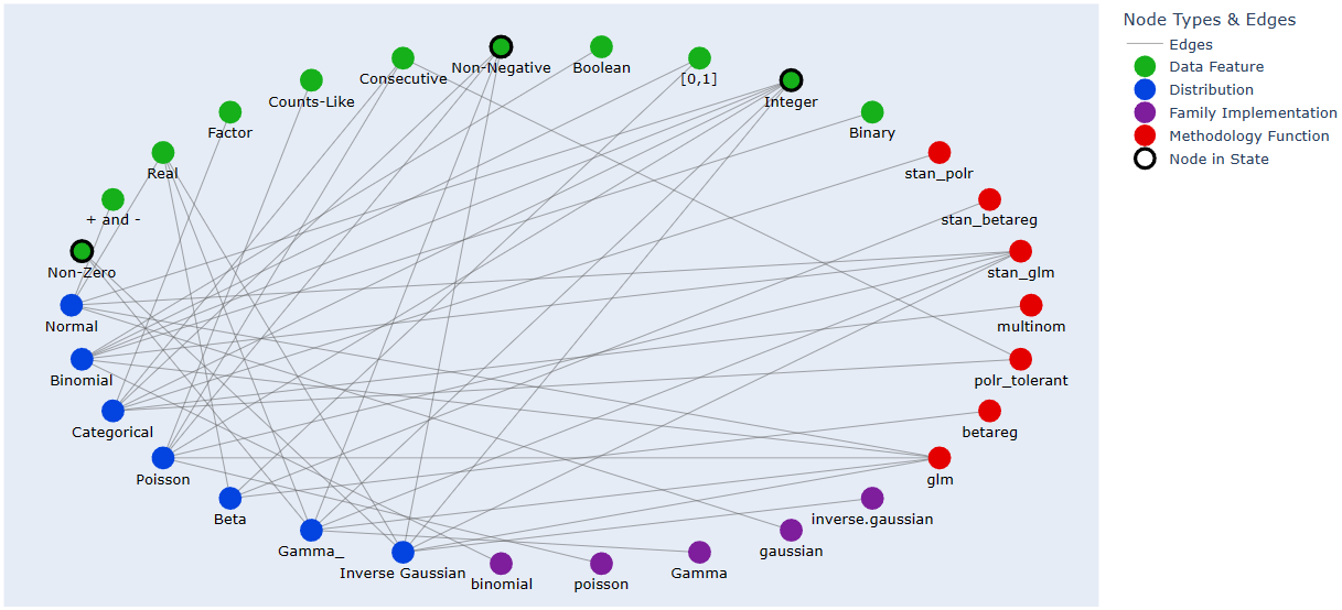
# gsm.plot(layout = nx.shell_layout, radial_labels = True) # Some other layout
# gsm.plot(plotly = False, show_necessity = False, show_sufficiency = True) # Networkx's native plotting backend instead of Plotly

gsm.consecutive_steps(dict(candidate_types = ['Distribution']), dict(candidate_types = ['Family Implementation']))
    # Perform 2 steps, providing named arguments (in this case only one) to the Scanner function as a dictionary

# gsm.consecutive_steps([['Distribution']], [['Family Implementation']]) # Unnamed-arguments version of the above
# gsm.parallel_steps([['Distribution']], [['Family Implementation']]) # Parallel version, warning of failure for 'Family Implementation'

print(gsm.log[-2], '\n') # Can check the log for details of the second-last step, where a tie occurs.
                         # Ties are rare, and the default Updater only picks one result, but arbitrary action may be taken

print(gsm._scan(['Methodology Function']), '\n') # Can also peek at the intermediate value of a step without going through with it
gsm.step(['Methodology Function']) # Perform the step (unnamed-Scanner-arguments version)

gsm.step(['NON EXISTING TYPE']) # Trigger a warning and no State changes
print(gsm.log[-1], '\n') # The failed step is also logged

print(gsm) # Prints the GSM State
The 'Methodology Function' scan above is peeked at before its step to show that there is a tie between a Frequentist and a Bayesian method.
This is a trivial example (in that the simple addition could have been there from the beginning) of where a broader graph could be attached by gsm.extend_with(...) and new state introduced in order to resolve the tie.
Note that ties need not really be resolved as long as the Updater function's behaviour is what the user expects since it is not limited in functionality; it could select a random option, all, some or none of them, it could adjust the graph itself or terminate execution.
See the Tests/self_contained_showcase_dict_state.py and Tests/self_contained_showcase_nec_suff.py files for slightly different versions of the above (the former with a state which is not a simple liest, and the latter with a graph including necessity and sufficiency relationships).
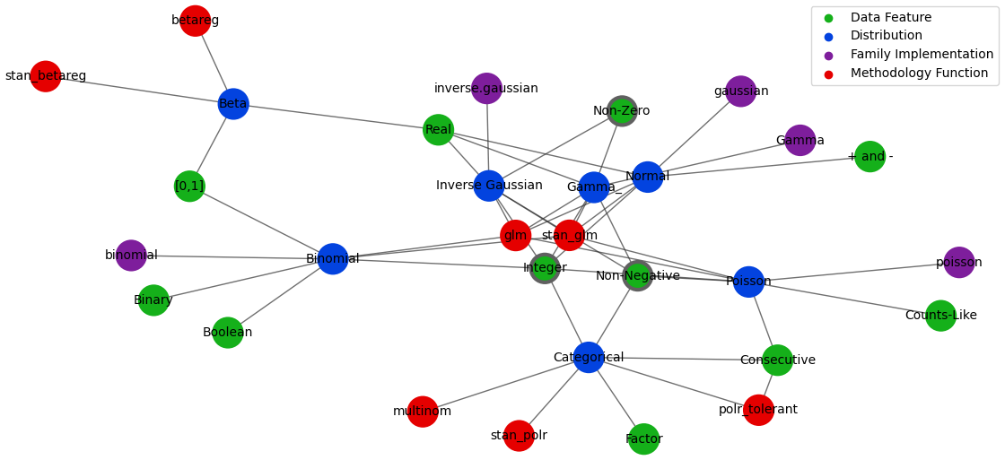
The default plot layout is Kamada-Kawai, and the default backend is Plotly (as in the image above), but arbitrary layouts can be provided, and the NetworkX-generated pyplot plotting is also available. Here are some alternative plotting possibilities:
