Codes for csLFM PSF conversion and 3D reconstruction
Version: 1.0
Lisence: GNU General Public License v2.0
We develop a confocal scanning light-field microscopy (csLFM), which synchronously employs scanning light-sheet illumination and a camera rolling shutter to selectively collect in-focus fluorescence upon a basic scanning LFM (sLFM) [paper]. By introducing simple modifications in the illumination path, csLFM enables high-sensitivity imaging with orders-of-magnitude reduction in background and the ability to resolve more subcellular details. After the acquisition of confocal scanning light-field images, iterative tomography with DAO, the same 3D reconstruction module as implemented in sLFM, is applied to obtain background-rejected, high-resolution volumes, with an accurately modelled point spread function (PSF) of csLFM.
This work mainly involves hardware innovations and physical propagation derivations. To enhance the ease of use of csLFM, we open-source this code package that is used for data processing after csLFM acquisiyion, including csLFM PSF generation and iterative 3D reconstructions. We also provides sLFM PSF, data and codes for the comparison.
More details please refer to the companion paper where this method first occurred [paper]. Next, we will guide you step by step to implement the csLFM PSF and reconstruction.
- a). 128 GB memory or better
- b). 1 NVIDIA GeForce RTX 3090 GPU or better
- Run the demo code named
main_for_sLFM_reconstruction3D.musing MATLAB. - The raw spatial-angular views captured by csLFM should be stored as
Data/csLFM_WDF.tif. Here, we provide a mouse brainslice data as demo. - The corresponding PSF file has been provided in the folder of
PSF. - The PSF should be firstly converted into the confocal one through line confocal modulation, which would be performed automatically in the
main_for_sLFM_reconstruction3D.m. - The final reconstruction results can be found in
Data/csLFM_Reconstruction.tif.
- Run the demo code named
main_for_sLFM_reconstruction3D.musing MATLAB. - The raw spatial-angular views captured by sLFM should be stored as
Data/sLFM_WDF.tif. Here, we provide the same mouse brainslice captured by sLFM as demo. - The corresponding PSF file has been provided in the folder of
PSF. - The final reconstruction results can be found in
Data/sLFM_Reconstruction.tif.
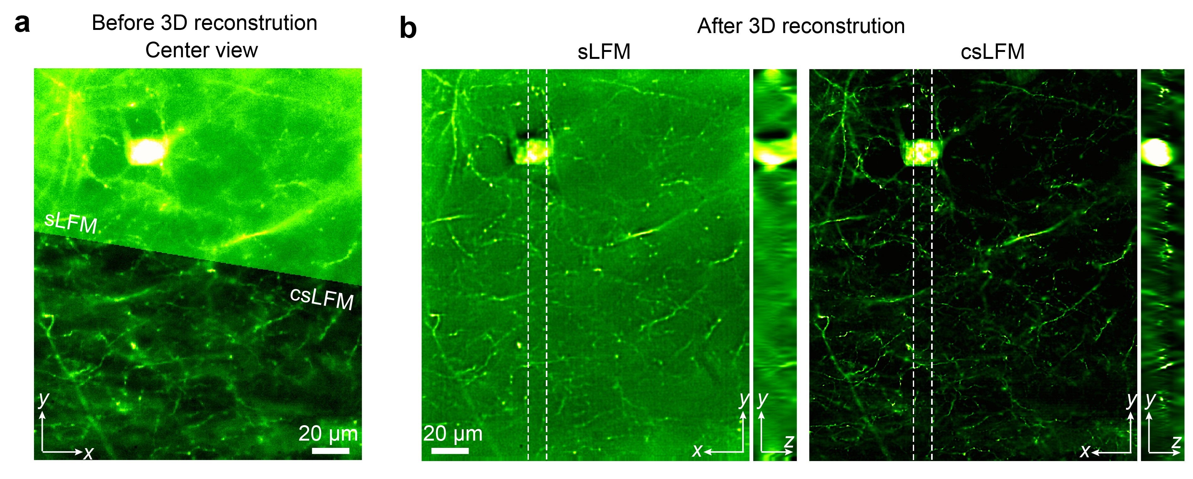
The centerviews and orthogonal average intensity projections of a YFP-labelled mouse brainslice by sLFM and csLFM are exhibited below. The white dashed lines indicate the regions for yz projection. For more results and further analysis, please refer to the companion paper where this method first occurred [paper]
If you use this code and relevant data, please cite the corresponding paper where original methods appeared:
Should you have any questions regarding this codes and the corresponding results, please contact Zhi Lu (luzhi@tsinghua.edu.cn).
