- CSC 461 PROJECT REPORT
- INTRODUCTION
- NECESSARY IMPORTS
- DATA COLLECTION
- DATA CLEANING
- Computing Raw Setnence Embeddings
- Previous Experiments
- Alignment Classification with Neural Networks
Our project delves into the synergy of machine learning and psychoanalysis, focusing on classifying sentences as either aligned with or divergent from Sigmund Freud's groundbreaking theories. Freud, the trailblazer in psychology, introduced concepts like the id, ego, and superego, shaping our understanding of the human mind.
By leveraging advanced natural language processing, our goal is to build models capable of discerning linguistic patterns associated with Freudian principles. This interdisciplinary exploration aims to unveil connections between language and psychological frameworks, contributing not only to psychology but also to the broader discourse on culture and language. Join us on this intellectual journey where machine learning meets psychoanalysis to uncover hidden dimensions of human expression and thought.
Initially, the content was scanned and read as a PDF document. Following this, the data underwent a transformation process, where it was structured and stored in a JSON (JavaScript Object Notation) file. This digital representation was meticulously organized to reflect the hierarchical structure of the original text.
In the JSON file, each chapter of Freud's works was designated as a separate array. Within these arrays, individual sentences from the chapters were indexed, thereby preserving the original sequence and organization of the text. This methodical approach not only facilitated the digitization of Freud's works but also ensured that the data remained accessible and easy to navigate in its new digital format.
A meticulous manual cleaning process was undertaken to refine the dataset. This stage involved the careful elimination of extraneous texts, ensuring the retention of only those works central to Sigmund Freud's oeuvre. The rationale behind this selective approach was to focus exclusively on Freud's principal publications, thereby enhancing the academic utility of the dataset.
Concurrently, the data structure of the JSON file underwent a transformation to better represent the hierarchical organization of the content. In this revised format, the titles of Freud's books were assigned as primary keys. Nested within these primary keys, each chapter title was designated as a subkey. These subkeys then encapsulated arrays, with each array element corresponding to an individual sentence from the respective chapter. This arrangement facilitated a more intuitive and accessible representation of the text.
It is noteworthy that for shorter works in Freud's collection, which lacked distinct chapter divisions, a singular subkey was employed. This subkey was named identically to the book title, and it contained an array of sentences representing the entire text of the work. This special consideration for shorter works ensured consistency and coherence in the organization of the digital archive, making it a comprehensive and systematically structured resource for scholarly research in psychoanalysis.
- "The Ego and the Id" (1940)
- "Some Elementary Lessons in Psycho-Analysis" (1940)
- "Splitting of the Ego in the Process of Defence" (1940)
- "Constructions in Analysis" (1937)
- "Analysis Terminable and Interminable" (1937)
- "An Outline of Psycho-Analysis" (1940)
- "Moses and Monotheism: Three Essays" (1939)
- "The Acquisition and Control of Fire" (1932)
- "Female Sexuality" (1931)
- "A Religious Experience" (1928)
- "Fetishism"
- "Humor"
- "Civilization and Its Discontents" (1930)
- "The Future of an Illusion"
- "Psycho-Analysis" (1926)
- "Inhibitions, Symptoms, and Anxiety" (1926)
- "Josef Popper-Lynkeus and the Theory of Dreams" (1923)
- "A Note Upon the Mystic Writing-Pad" (1925)
- "A Short Account of Psycho-Analysis" (1924)
- "The Infantile Genital Organization (An Interpolation into the Theory of Sexuality)" (1923)
- "Remarks on the Theory and Practice of Dream-Interpretation" (1923)
- "A Seventeenth-Century Demonological Neurosis" (1923)
- "Two Encyclopaedia Articles" (1923)
- "Dreams and Telepathy" (1922)
- "Psycho-Analysis and Telepathy" (1941 [1921])
- "Group Psychology and the Analysis of the Ego" (1921)
- "Beyond the Pleasure Principle" (1920)
- "On the History of the Psycho-Analytic Movement" (1914)
- "The Uncanny" (1919)
- "The Moses of Michelangelo" (1914)
- "Observations and Examples from Analytic Practice" (1913)
- "The Claims of Psycho-Analysis to Scientific Interest" (1913)
- "Introduction to Pfister's The Psycho-Analytic Method" (1913)
- "The Disposition to Obsessional Neurosis: A Contribution to the Problem of Choice of Neurosis" (1913)
- "Two Lies Told by Children" (1913)
- "The Occurrence in Dreams of Material from Fairy Tales" (1913)
- "An Evidential Dream" (1913)
- "Types of Onset of Neurosis" (1912)
- "A Note on the Unconscious in Psycho-Analysis" (1912)
- "Wild Psycho-Analysis" (1910)
- "Formulations on the Two Principles of Mental Functioning" (1911)
- "Five Lectures on Psycho-Analysis" (1910)
- "Some General Remarks on Hysterical Attacks" (1909)
- "Family Romances" (1909)
- "On the Sexual Theories of Children" (1908)
- "Notes upon a Case of Obsessional Neurosis" (1909)
- "The Sexual Enlightenment of Children (An Open Letter to Dr. M. Frst)" (1907)
- "My Views on the Part Played by Sexuality in the Aetiology of the Neuroses" (1906)
- "Three Essays on the Theory of Sexuality" (1905)
- "Freud's Psycho-Analytic Procedure" (1904)
- "On Psychotherapy" (1905)
- "The Psychopathology of Everyday Life"
- "Fragment of an Analysis of a Case of Hysteria (1905 [1901])"
- "On Dreams" (1901)
- "The Interpretation of Dreams" (1900)
- "The Psychical Mechanism of Forgetfulness" (1898)
- "Screen Memories" (1899)
- "Sexuality in the Aetiology of the Neuroses" (1898)
- "Abstracts of the Scientific Writings of Dr. SigM. Freud 1877-1897" (1897)
- "The Aetiology of Hysteria" (1896)
- "Further Remarks on the Neuro-Psychoses of Defence" (1896)
- "Heredity and the Aetiology of the Neuroses" (1896)
- "A Reply to Criticisms of My Paper on Anxiety Neurosis"
- "Obsessions and Phobias"
- "On the Grounds for Detaching a Particular Syndrome from Neurasthenia Under the Description Anxiety Neurosis"
- "Charcot"
- "The Neuro-Psychoses of Defence"
- "Studies on Hysteria" (1893-1895)
with open("Cleaned_data.json") as file:
    train_data = json.load(file)
dict_data = {
"sentence": [],
"class": []
}Here, an empty dictionary dict_data is initialized with two keys: "sentence" and "class". These keys will be used to store sentences and their associated class labels, respectively.
for book, chapters in train_data.items():
    for chapter, sentences in chapters.items():
        for sentence in sentences:
            dict_data["sentence"].append(sentence)
            dict_data["class"].append(1)

train_df = pd.DataFrame(dict_data)
print(train_df.head())
train_df.to_csv("dataset.csv")
In this loop, the code iterates through each book and chapter in train_data. For every sentence found in each chapter, the sentence is appended to the dict_data["sentence"] list, and a corresponding class label '1' is appended to the dict_data["class"] list. This operation effectively flattens the hierarchical structure of the data into a format suitable for tabular analysis.
def drop_rows_with_integer_in_first_column(csv_file):
    df = pd.read_csv(csv_file)
    first_column = df.iloc[:, 1]
    def is_integer(value):
        try:
            int(value)
            return True
        except ValueError:
            return False

    non_integer_mask = ~first_column.apply(is_integer)
    filtered_df = df[non_integer_mask]

    return filtered_df

filtered_df = drop_rows_with_integer_in_first_column("dataset.csv")
Further step of cleaning removing rows that have pure integer value in the column "Sentence"
no_df = pd.read_csv("tweet_emotions.csv")

no_df["class"] = 0

no_df = no_df[["content", "class"]]

no_df.rename(columns={'content': 'sentence'}, inplace=True)

final_df = pd.concat([filtered_df, no_df]).reset_index(drop=True)

final_df.to_csv("final_dataset.csv")
Finally we used a random dataset that we found on kaggle to ensure that our model, trained to identify sentences relevant to Freud's concepts and maintains a high degree of accuracy and specificity. By introducing this heterogeneous set of sentences, we aimed to rigorously test and validate the model's capability to accurately distinguish between relevant and non-relevant content, thereby mitigating the risk of misclassification of contextually unrelated sentences as being associated with Freudian theories.
In the approach described, the all-MiniLM-L6-v2 language model used for computing sentence embeddings with SentenceBERT was developed by the research team at Microsoft. This model is a part of the MiniLM series, which is known for providing high-quality language representations while being more efficient and compact compared to larger models
The SentenceTransformer model is initialized with the all-MiniLM-L6-v2 model.
We then encode the sentences present in the DataFrame df, under the column 'sentence'.
The resulting embeddings are stored in the variable sbert_embeddings.
Finally, these embeddings are saved to a file named "embeddings_v0.npy" for future use or analysis.
Checking the shape of the embeddings array gives us insight into the dimensions of the dataset in the embedded space.
sbert_embeddings.shape(93104, 384)
The output (93104, 384) indicates the transformation of 93,104 sentences into a 384-dimensional embedding space. Each of these dimensions encapsulates complex semantic features of the sentences, now rendered in a numerical format suitable for NLP applications.
The generated sentence embeddings are then saved for future use, as we can simply load them back instead of having to recompute them every time.
np.save("embeddings_v0.npy", sbert_embeddings)We employ the Word2Vec methodology, a widely recognized technique in the field of Natural Language Processing (NLP), for generating word embeddings.
The initial stage involves preprocessing the data to make it suitable for training the Word2Vec model. This step includes tokenizing the sentences in our dataset. Tokenization is the process of breaking down text into smaller units, typically words. Each sentence in the dataset is split into a list of words, facilitating the subsequent training of the Word2Vec model.
Once preprocessing is complete, we proceed to train the Word2Vec model on the tokenized data. The training process involves configuring several parameters that influence the model's performance and the quality of the word embeddings
We pass the Word2Vec model:
datawhich is our corpus of sentenceswindowwhich refers to the "window" of words, as in the number of words before and after the target word that the model will use as context to learn the targetmin_countreferring to the minimum frequency the word should have to be considered in the model's dictionaryworkersspecifying the number of threads the model will use to train.
After training the Word2Vec model and extracting word embeddings, the next significant step is to create sentence embeddings. Sentence embeddings represent the entire sentence in a vectorized form and are vital for tasks where the semantic understanding of the whole sentence is required.
The sentence_embedding function outlined below is designed to generate a vector representation of a sentence. This function operates by first checking if the input is numerical (float or int), returning a zero vector in such cases to handle missing or non-textual data. For textual inputs, the function tokenizes the sentence into individual words, retrieves their corresponding embeddings from the trained Word2Vec model, and then computes the average of these word embeddings. This average vector serves as the embedding for the entire sentence.
The dimensionality of each sentence embedding is set to 384, consistent with our model's configuration. If a sentence does not contain any words present in our Word2Vec vocabulary, a zero vector of size 384 is returned.
In this section, we will discuss our initial experimentation with computing sentence similarity and basing our classification on that. This type of thinking, while it seemed interesting, did not yeild good enough results.
For this task, our data was comprised of the sentences from Freud's books that we would compute embeddings for using the schemes defined above. We considered the classes as books, meaning a sentence is to be classified by the book it came from. One proposition we had was to use the chapters as classes, but that would mean having 233 total classes which is a lot and did in reality cause problems in our earlier experiments.
def euclidean(p1, p2):
    dist = np.sqrt(np.sum(p1-p2)**2)
    return dist
It calculates the Euclidean distance between two points in a multi-dimensional space,for quantifying the dissimilarity between data points.
def filter_by_threshold_cos(scores, threshold, k):
    new_k = k
    if scores[0]["score"] < threshold:
        return []
    else:
        top_k = scores[:k]
        for i, s in enumerate(top_k):
            if s["score"] < threshold:
                new_k = i
                break
        return scores[:new_k]
This function is an implementation of a threshold-based selection algorithm for cosine similarity scores. It strategically filters a list of scores, retaining only the top k scores that surpass a specified similarity threshold.
def filter_by_threshold_euclidean(distances, threshold, k):
    new_k = k
    if distances[0]["dist"] > threshold:
        return []
    else:
        top_k = distances[:k]
        for i, d in enumerate(top_k):
            if d["dist"] > threshold:
                new_k = i
                break
        return distances[:new_k]
Comparable in certain respects to the cosine similarity filtering function, this variant is tailored for contexts involving Euclidean distances. It selectively retains the top k elements from a set of distances, adhering to a predefined Euclidean distance threshold.
ALIGNMENT_THRESHOLD_COS = 0.6
ALIGNMENT_THRESHOLD_EUC = 1
MISALIGNMENT_STRING = "This sentence does not align with any of Freud's ideas"
ALIGNMENT_THRESHOLD_COS and ALIGNMENT_THRESHOLD_EUC: These constants represent the predefined thresholds for cosine similarity and Euclidean distance, respectively. They are integral to the filtering operations within the classification framework.
Essentially, we proposed two main methods with slight variations.
Our first approach is similar to performing KNN; given an input sentence, we can compute its embedding, then we can get the closest other sentences to it that exist in the embedding space (ie exist in the "training" sentences) and then we can have a voting mechanism between these
Our second approach entails computing the centroids of each cluster of embeddings corresponding to a class of sentences, then we can perform compute distance/similarity between the input sentence's embeddings and the centroids of the classes, and we consider the closest centroid the right class.
In both cases, the distance/similarity can either be using traditional euclidean distance, or cosine similarity. In our experiments, we try both approaches and try to compare them.
Below is a function we created to modularize the testing process:
def modular_predict(incoming_embedding, training_embeddings, sim_score, choice_mode, train_df, k = None):
    if sim_score == "cos":
        if choice_mode == "knn":
            cos_sim_score = util.cos_sim(incoming_embedding, training_embeddings)
            pairs = []
            sentences = list(train_df["sentence"])
            for i, sen in enumerate(sentences):
                pairs.append({'index': i, 'score': cos_sim_score[:, i]})
            pairs = sorted(pairs, key=lambda x: x['score'], reverse=True)
            top_pairs = filter_by_threshold_cos(pairs, ALIGNMENT_THRESHOLD_COS, k)
            top_mask = [pair["index"] for pair in top_pairs]
            top_classes = list(train_df["class"][top_mask])
            if len(top_classes) == 0:
                return MISALIGNMENT_STRING
            counter = Counter(top_classes)
            freqs = {k: v for k, v in counter.items()}
            lab = max(freqs, key=freqs.get)
            return lab

        elif choice_mode == "centroid":
            class_reps = {}
            unique_classes = train_df["class"].unique()
            for class_name in unique_classes:
                mask = train_df["class"] == class_name
                embs = training_embeddings[mask]
                avg_embedding = np.mean(embs, axis=0)
                class_reps[class_name] = avg_embedding
            cos_score = util.cos_sim(incoming_embedding, list(class_reps.values()))
            x = list(cos_score[0,:])
            cos_score = [float(y) for y in x]
            class_score = list(zip(unique_classes, cos_score))
            results = sorted(class_score, key=lambda x: x[1], reverse=True)
            if results[0][1] < ALIGNMENT_THRESHOLD_COS:
                return MISALIGNMENT_STRING
            else:
                return results[0][0]

    elif sim_score == "euclidean":
        if choice_mode == "knn":
            dist_to_all = []
            pairs = []
            for j in range(len(training_embeddings)):
                distance = euclidean(np.array(training_embeddings[j,:]), incoming_embedding)
                dist_to_all.append(distance)
            sentences = list(train_df["sentence"])
            for i, sen in enumerate(sentences):
                pairs.append({'index': i, 'dist': dist_to_all[i]})
            # print min and max distances
            # print(min(dist_to_all), " - ", max(dist_to_all))
            pairs = sorted(pairs, key=lambda x: x['dist'], reverse=False)
            top_pairs = filter_by_threshold_euclidean(pairs, ALIGNMENT_THRESHOLD_EUC, k)
            top_mask = [pair["index"] for pair in top_pairs]
            top_classes = list(train_df["class"][top_mask])
            if len(top_classes) == 0:
                return MISALIGNMENT_STRING
            counter = Counter(top_classes)
            freqs = {k: v for k, v in counter.items()}
            lab = max(freqs, key=freqs.get)
            return lab


        elif choice_mode == "centroid":
            class_reps = {}
            unique_classes = train_df["class"].unique()
            for class_name in unique_classes:
                mask = train_df["class"] == class_name
                embs = training_embeddings[mask]
                avg_embedding = np.mean(embs, axis=0)
                class_reps[class_name] = avg_embedding
            distances = [euclidean(incoming_embedding, emb) for emb in list(class_reps.values())]
            cbe_pairs = list(zip(list(class_reps.keys()), distances))
            cbe_results = sorted(cbe_pairs, key=lambda x: x[1], reverse=True)
            if cbe_results[0][1] < ALIGNMENT_THRESHOLD_COS:
                return MISALIGNMENT_STRING
            else:
return cbe_results[0][0]def evaluate(input_sentences, model, model_type, sim_score, choice_mode, training_embeddings, train_df, k = None):
"""
Predicts classification of inputs sentences and returns a summary of metrics
Args:
input_sentences: sentences that we want to classify
model: model object
model_type: `word2vec` or `sbert`
sim_score: `cos` or `euclidean`
choice_mode: `knn` or `centroid`
training_embeddings: embeddings of the training corpus
train_df: dataframe containing the csv data
k: k for knn
"""
predicted_classes = []
true_classes = list(input_sentences.values())
for sentence, klass in input_sentences.items():
if model_type == "sbert":
input_embedding = model.encode(sentence)
elif model_type == "word2vec":
words = sentence.split()
word_embeddings = [model.wv[word] for word in words if word in model.wv]
if len(word_embeddings) == 0:
return np.zeros(model.vector_size)
input_embedding = np.mean(word_embeddings, axis=0)
pred = modular_predict(input_embedding, training_embeddings, sim_score, choice_mode, train_df, k)
predicted_classes.append(pred)
accuracy = accuracy_score(true_classes, predicted_classes)
precision = precision_score(true_classes, predicted_classes, average='macro')
recall = recall_score(true_classes, predicted_classes, average='macro')
f1 = f1_score(true_classes, predicted_classes, average='macro')
conf_matrix = confusion_matrix(true_classes, predicted_classes)
print('Accuracy: %.3f' % accuracy)
print('Precision: %.3f' % precision)
print('Recall: %.3f' % recall)
print('F1 Score: %.3f' % f1)
print('Confusion Matrix:')
print(conf_matrix)
return predicted_classescomputes and disseminates a suite of classification metrics including accuracy, precision, recall, F1 score, and a confusion matrix,
model = SentenceTransformer('all-MiniLM-L6-v2')embeddings = np.load("sbert_embeddings_v1.npy")
evaluate(small, model, "sbert", "cos", "knn", embeddings, df, 5)
results = evaluate(small, model, "sbert", "cos", "centroid", embeddings, df, 5)The decision to move away from the current model was made because it wasn't performing well and we didn't have enough time to figure out and fix the issues. This led us to look for a different model that could potentially work better within our time constraints.
We decided to take a different approach here, and treat the embedding space as tabular data, such that the number of dimensions is equivalent to the "number of columns" tabular data would have, ie. every dimension would be a feature.
First, we extract a list of the labels for each observation in our dataset. We also assume we have the embeddings ready from either SBERT or word2vec as a variable embeddings
labels = np.array(list(df["class"]))Next, we split our dataset into training and testing splits with 20% of our data for testing and 80% for training. Additionally, we specify a random state of 42 to ensure reproducability
X_train, X_test, y_train, y_test = train_test_split(embeddings, labels, test_size=0.2, random_state=42)We tried a variety of architectures, below you can see an example of our nn_shallow_9310.h5 model.
The Rectified Linear Unit and Sigmoid Functions, can be modeled by:
The rest of the models work very similarly with all hidden layers employing the relu function as a activation function to add non-linearity and the final layer using sigmoid because we're doing binary classification (we would probably have better results using softmax for multiclass classification for example)
After that, we compile our model as is required by TensorFlow (the backend used by Keras in our case). In this step we can specify:
binary_crossentropy: the loss function that the model will use during training. This loss function is commonly used for binary classification problems where the output of the model is a probability distribution over two classesadam: the optimization algorithm used to update the weights of the neural network during training. Adam is also the most popular algorithm in this field for neural networksaccuracy: metric used to evaluate the performance of the model
Here, we train our models, all given the same data, and trained over 10 epochs with a batch size of 32.
We did not need more than 10 epochs as is evident by our high accuracy reported below, so we did not raise the number of epochs to avoid overfitting, but at the same time, we kept it this high so we can learn as much as possible.
For each model we trained, we kept track of most important classification metrics like:
- Accuracy
- Precision
- Recall
- F1 Score
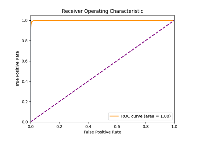
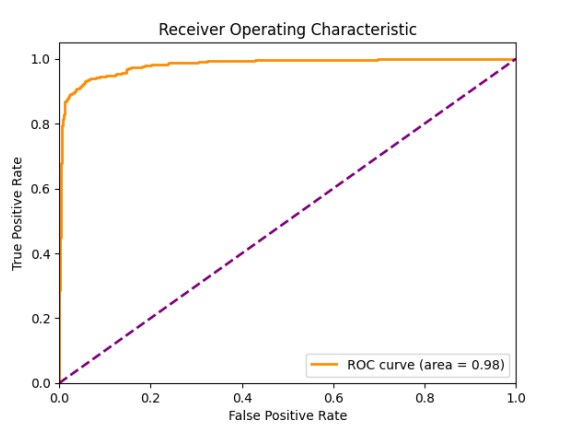
- AUC
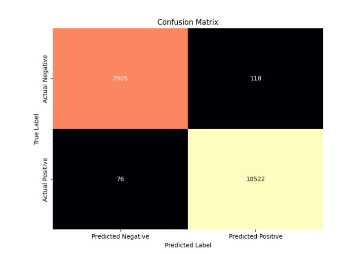
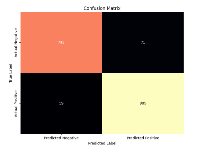
We also computed the Confusion Matrices for the models to better understand the nature of the errors our models made.
First, we use the model to predict on our test set, then we convery the probability outputs into binary classifications and get the all the metrics
Our best performing model was nn_sbert_93k with the following metrics:
| Accuracy | Precision | Recall | F1 | AUC |
|---|---|---|---|---|
| 0.99 | 0.99 | 0.989 | 0.989 | 1.0 |
Meanwhile, our worst performing model was small_nn_w2v_9k with the following metrics:
| Accuracy | Precision | Recall | F1 | AUC |
|---|---|---|---|---|
| 0.93 | 0.93 | 0.928 | 0.929 | 0.98 |
Here is the complete list of the configurations we ran for our models:
 In general, we see a trend where training models with the same architecture on SBERT embeddings yielded better results than those of
 word2vec, and we also see a direct positive relationship between the size of the training data and the average performance of the model.


