The sjSDM package is an R package for estimating joint species distribution models. A jSDM is a GLMM that models a multivariate (i.e. a many-species) response to the environment, space and a covariance term that models conditional (on the other terms) correlations between the outputs (i.e. species).
imageA big challenge in jSDM implementation is computational speed. The goal of the sjSDM (which stands for “scalable joint species distribution models”) is to make jSDM computations fast and scalable. Unlike many other packages, which use a latent-variable approximation to make estimating jSDMs faster, sjSDM fits a full covariance matrix in the likelihood, which is, however, numerically approximated via simulations. The method is described in Pichler & Hartig (2021) A new joint species distribution model for faster and more accurate inference of species associations from big community data, https://www.doi.org/10.1111/2041-210X.13687.
The core code of sjSDM is implemented in Python / PyTorch, which is then wrapped into an R package. In principle, you can also use it stand-alone under Python (see instructions below). Note: for both the R and the python package, python >= 3.7 and pytorch must be installed (more details below). However, for most users, it will be more convenient to use sjSDM via the sjSDM R package, which also provides a large number of downstream functionalities.
To get citation info for sjSDM when you use it for your reseach, type
citation("sjSDM")sjSDM is distributed via CRAN. For most users, it will be best to install the package from CRAN
install.packages("sjSDM")Depencies for the package can be installed before or after installing the package. Detailed explanations of the dependencies are provided in vignette(“Dependencies”, package = “sjSDM”), source code here. Very briefly, the dependencies can be automatically installed from within R:
sjSDM::install_sjSDM(version = "gpu") # or
sjSDM::install_sjSDM(version = "cpu")
For advanced users: if you want to install the current (development) version from this repository, run
devtools::install_github("https://github.com/TheoreticalEcology/s-jSDM", subdir = "sjSDM", ref = "master")dependencies should be installed as above. If the installation fails, check out the help of ?install_sjSDM, ?installation_help, and vignette(“Dependencies”, package = “sjSDM”).
- Try install_sjSDM()
- New session, if no ‘PyTorch not found’ appears it should work, otherwise see ?installation_help
- If do not get the pkg to run, create an issue issue tracker or write an email to maximilian.pichler at ur.de
Load the package
library(sjSDM)Simulate some community data
set.seed(42)
community <- simulate_SDM(sites = 100, species = 10, env = 3, se = TRUE)
Env <- community$env_weights
Occ <- community$response
SP <- matrix(rnorm(200, 0, 0.3), 100, 2) # spatial coordinates (no effect on species occurences)
This fits the standard SDM with environmental, spatial and covariance terms
model <- sjSDM(Y = Occ, env = linear(data = Env, formula = ~X1+X2+X3), spatial = linear(data = SP, formula = ~0+X1:X2), se = TRUE, family=binomial("probit"), sampling = 100L, verbose = FALSE)summary(model)## Family: binomial
##
## LogLik: -505.3381
## Regularization loss: 0
##
## Species-species correlation matrix:
##
## sp1 1.0000
## sp2 -0.3700 1.0000
## sp3 -0.1980 -0.4260 1.0000
## sp4 -0.1670 -0.3830 0.8330 1.0000
## sp5 0.6670 -0.3620 -0.1330 -0.1040 1.0000
## sp6 -0.2910 0.4780 0.1730 0.1860 -0.1020 1.0000
## sp7 0.5740 -0.1110 0.1270 0.1790 0.5370 0.2740 1.0000
## sp8 0.2870 0.2150 -0.5160 -0.5250 0.2000 -0.0060 0.1100 1.0000
## sp9 -0.0610 -0.0560 0.0510 0.0580 -0.3950 -0.3590 -0.2320 -0.1310 1.0000
## sp10 0.2050 0.5050 -0.7150 -0.6640 0.2550 0.1480 0.1380 0.4670 -0.2610 1.0000
##
##
##
## Spatial:
## sp1 sp2 sp3 sp4 sp5 sp6 sp7 sp8
## X1:X2 2.10835 -4.061843 3.446407 0.4750172 2.757261 0.9577488 3.384754 2.053963
## sp9 sp10
## X1:X2 1.003981 1.293782
##
##
##
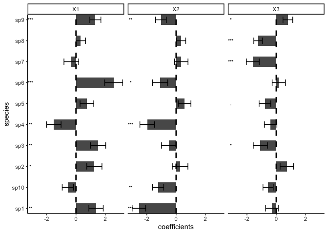
## Estimate Std.Err Z value Pr(>|z|)
## sp1 (Intercept) -0.1038 0.2614 -0.40 0.69129
## sp1 X1 1.3685 0.4894 2.80 0.00517 **
## sp1 X2 -2.5386 0.4626 -5.49 4.1e-08 ***
## sp1 X3 -0.2941 0.4331 -0.68 0.49713
## sp2 (Intercept) -0.0106 0.2760 -0.04 0.96949
## sp2 X1 1.2541 0.5173 2.42 0.01534 *
## sp2 X2 0.2723 0.5312 0.51 0.60824
## sp2 X3 0.7237 0.4605 1.57 0.11603
## sp3 (Intercept) -0.5153 0.2854 -1.81 0.07100 .
## sp3 X1 1.5114 0.5174 2.92 0.00349 **
## sp3 X2 -0.4924 0.5080 -0.97 0.33235
## sp3 X3 -1.0819 0.4862 -2.23 0.02606 *
## sp4 (Intercept) -0.0771 0.2559 -0.30 0.76318
## sp4 X1 -1.5116 0.4940 -3.06 0.00222 **
## sp4 X2 -1.9738 0.4985 -3.96 7.5e-05 ***
## sp4 X3 -0.3837 0.4295 -0.89 0.37164
## sp5 (Intercept) -0.2368 0.2424 -0.98 0.32864
## sp5 X1 0.7438 0.4670 1.59 0.11121
## sp5 X2 0.5777 0.4317 1.34 0.18081
## sp5 X3 -0.7728 0.3984 -1.94 0.05244 .
## sp6 (Intercept) 0.3047 0.2753 1.11 0.26847
## sp6 X1 2.5735 0.6142 4.19 2.8e-05 ***
## sp6 X2 -1.0934 0.5190 -2.11 0.03513 *
## sp6 X3 0.1742 0.4538 0.38 0.70103
## sp7 (Intercept) -0.0224 0.2574 -0.09 0.93054
## sp7 X1 -0.3184 0.5029 -0.63 0.52667
## sp7 X2 0.3480 0.4616 0.75 0.45090
## sp7 X3 -1.5991 0.4387 -3.64 0.00027 ***
## sp8 (Intercept) 0.1415 0.1673 0.85 0.39759
## sp8 X1 0.3254 0.3263 1.00 0.31864
## sp8 X2 0.3401 0.3154 1.08 0.28092
## sp8 X3 -1.2411 0.2907 -4.27 2.0e-05 ***
## sp9 (Intercept) 0.0200 0.1955 0.10 0.91852
## sp9 X1 1.3218 0.3775 3.50 0.00046 ***
## sp9 X2 -1.0367 0.3700 -2.80 0.00508 **
## sp9 X3 0.7911 0.3337 2.37 0.01775 *
## sp10 (Intercept) -0.0983 0.2091 -0.47 0.63821
## sp10 X1 -0.5550 0.3861 -1.44 0.15064
## sp10 X2 -1.2310 0.3852 -3.20 0.00139 **
## sp10 X3 -0.5567 0.3514 -1.58 0.11315
## ---
## Signif. codes: 0 '***' 0.001 '**' 0.01 '*' 0.05 '.' 0.1 ' ' 1
Plot the niche estimates, i.e the estimates in the environmental component:
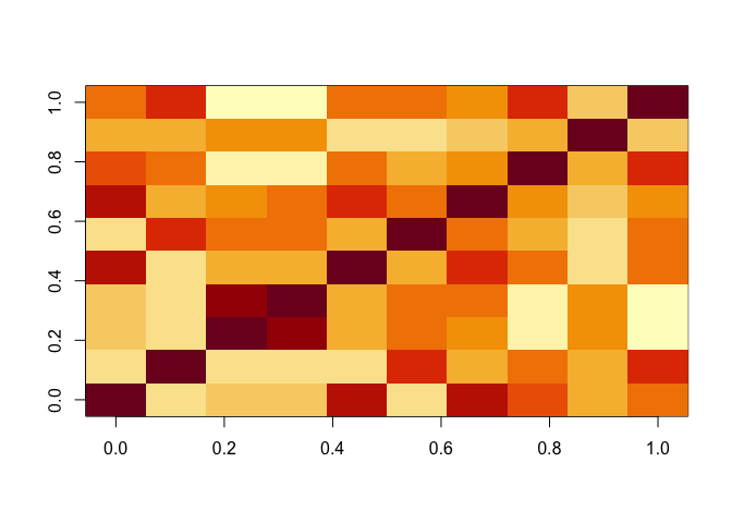
plot(model)Visualize the species-species association matrix
image(getCor(model))As in other models, it can be interesting to analyze how much variation is explained by which parts of hte model.
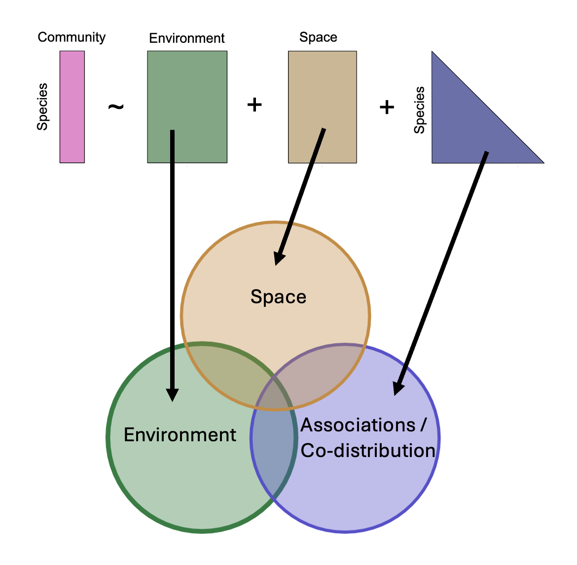 {{width=70%}} For the Env,
Spatial, Covariance terms, this is implemented in
an = anova(model, verbose = FALSE)summary(an)## Analysis of Deviance Table
##
## Deviance Residual deviance R2 Nagelkerke
## Abiotic 194.588270 1123.695071 0.857139
## Associations 209.748671 1108.534671 0.877235
## Spatial 9.507160 1308.776181 0.090692
## Shared Abiotic+Associations -34.334444 1352.617785 -0.409654
## Shared Abiotic+Spatial 4.358766 1313.924576 0.042651
## Shared Spatial+Associations 8.218556 1310.064785 0.078899
## Shared Abiotic+Associations+Spatial -23.674394 1341.957736 -0.267117
## Full 368.412583 949.870758 0.974881
## R2 McFadden
## Abiotic 0.1421
## Associations 0.1532
## Spatial 0.0069
## Shared Abiotic+Associations -0.0251
## Shared Abiotic+Spatial 0.0032
## Shared Spatial+Associations 0.0060
## Shared Abiotic+Associations+Spatial -0.0173
## Full 0.2691
plot(an)The anova shows the relative changes in the R2 of the groups and their intersections.
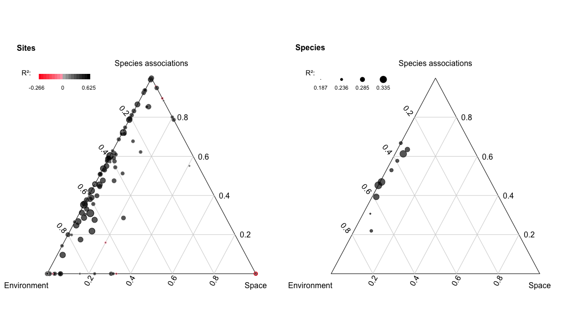
Following Leibold et al., 2022 we can calculate and visualize the internal metacommunity structure (=partitioning of the three components for species and sites). The internal structure is already calculated by the ANOVA and we can visualize it with the plot method:
results = internalStructure(an) # or plot(an, internal = TRUE)The plot function returns the results for the internal metacommunity structure:
plot(results)## Registered S3 methods overwritten by 'ggtern':
## method from
## grid.draw.ggplot ggplot2
## plot.ggplot ggplot2
## print.ggplot ggplot2
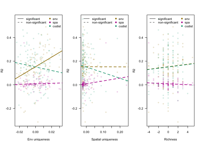
Which can be regressed against covariates to analyse assembly processes:
plotAssemblyEffects(results)If you want to use sjSDM from python (as said, not encouraged because all help and downstream functions are in R), install via
pip install sjSDM_pyPython example
import sjSDM_py as fa
import numpy as np
import torch
Env = np.random.randn(100, 5)
Occ = np.random.binomial(1, 0.5, [100, 10])

model = fa.Model_sjSDM(device=torch.device("cpu"), dtype=torch.float32)
model.add_env(5, 10)
model.build(5, optimizer=fa.optimizer_adamax(0.001),scheduler=False)
model.fit(Env, Occ, batch_size = 20, epochs = 10)
# print(model.weights)
# print(model.covariance)
Calculate Importance:
Beta = np.transpose(model.env_weights[0])
Sigma = ( model.sigma @ model.sigma.t() + torch.diag(torch.ones([1])) ).data.cpu().numpy()
covX = fa.covariance( torch.tensor(Env).t() ).data.cpu().numpy()

fa.importance(beta=Beta, covX=covX, sigma=Sigma)


