Interpret-Community is an experimental repository extending Interpret, with additional interpretability techniques and utility functions to handle real-world datasets and workflows for explaining models trained on tabular data. This repository contains the Interpret-Community SDK and Jupyter notebooks with examples to showcase its use.
- Overview of Interpret-Community
- Getting Started
- Supported Models
- Supported Interpretability Techniques
- Use Interpret-Community
- Contributing
- Code of Conduct
Interpret-Community extends the Interpret repository and incorporates further community developed and experimental interpretability techniques and functionalities that are designed to enable interpretability for real world scenarios. Interpret-Community enables adding new experimental techniques (or functionalities) and performing comparative analysis to evaluate them.
Interpret-Community
- Actively incorporates innovative experimental interpretability techniques and allows for further expansion by researchers and data scientists
- Applies optimizations to make it possible to run interpretability techniques on real-world datasets at scale
- Provides improvements such as the capability to "reverse the feature engineering pipeline" to provide model insights in terms of the original raw features rather than engineered features
- Provides interactive and exploratory visualizations to empower data scientists to gain meaningful insight into their data
This repository uses Anaconda to simplify package and environment management.
To setup on your local machine:
1. Set up Environment
a. Install Anaconda with Python >= 3.6
   [Miniconda](https://conda.io/projects/conda/en/latest/user-guide/install/index.html) is a quick way to get started.


b. Create conda environment named interp and install packages
conda create --name interp python=3.6 anaconda
Optional, additional reading:
conda cheat sheet jupyter nb_conda
On Linux and Windows: c. Activate conda environment
activate interp
On Mac: c. Activate conda environment
source activate interp
2. Clone the Interpret-Community repository
Clone and cd into the repository
git clone https://github.com/interpretml/interpret-community
cd interpret-community
3. Install Python module, packages and necessary distributions
pip install interpret-community
If you intend to run repository tests:
pip install -r requirements.txt
On Windows:
Pytorch installation if desired:
    pip install https://download.pytorch.org/whl/cpu/torch-1.3.0%2Bcpu-cp36-cp36m-win_amd64.whl
    pip install torchvision==0.4.1
lightgbm installation if desired:
conda install --yes -c conda-forge lightgbm
On Linux:
Pytorch installation if desired: pip install torch==1.3.0
pip install torchvision==0.4.1
lightgbm installation if desired:
conda install --yes -c conda-forge lightgbm
On MacOS:
Pytorch installation if desired:
    pip install torch==1.3.0
    pip install torchvision==0.4.1
lightgbm installation if desired (requires Homebrew):
    brew install libomp
    conda install --yes -c conda-forge lightgbm
If installing the package generally gives an error about the certifi package, run this first:
    pip install --upgrade certifi --ignore-installed
    pip install interpret-community
4. Set up and run Jupyter Notebook server
Install and run Jupyter Notebook
if needed:
          pip install jupyter
then:
jupyter notebook
This API supports models that are trained on datasets in Python numpy.array, pandas.DataFrame, iml.datatypes.DenseData, or scipy.sparse.csr_matrix format.
The explanation functions accept both models and pipelines as input as long as the model or pipeline implements a predict or predict_proba function that conforms to the Scikit convention. If not compatible, you can wrap your model's prediction function into a wrapper function that transforms the output into the format that is supported (predict or predict_proba of Scikit), and pass that wrapper function to your selected interpretability techniques.
If a pipeline script is provided, the explanation function assumes that the running pipeline script returns a prediction. The repository also supports models trained via PyTorch, TensorFlow, and Keras deep learning frameworks.
The following are a list of the experimental explainers available in the community repository:
| Interpretability Technique | Description | Type |
|---|---|---|
| SHAP Kernel Explainer | SHAP's Kernel explainer uses a specially weighted local linear regression to estimate SHAP values for any model. | Model-agnostic |
| GPU SHAP Kernel Explainer | GPU Kernel explainer uses cuML's GPU accelerated version of SHAP's Kernel Explainer to estimate SHAP values for any model. It's main advantage is to provide acceleration to fast GPU models, like those in cuML. But it can also be used with CPU-based models, where speedups can still be achieved but they might be limited due to data transfers and speed of models themselves. | Model-agnostic |
| SHAP Tree Explainer | SHAP’s Tree explainer, which focuses on the polynomial time fast SHAP value estimation algorithm specific to trees and ensembles of trees. | Model-specific |
| SHAP Deep Explainer | Based on the explanation from SHAP, Deep Explainer "is a high-speed approximation algorithm for SHAP values in deep learning models that builds on a connection with DeepLIFT described in the SHAP NIPS paper. TensorFlow models and Keras models using the TensorFlow backend are supported (there is also preliminary support for PyTorch)". | Model-specific |
| SHAP Linear Explainer | SHAP's Linear explainer computes SHAP values for a linear model, optionally accounting for inter-feature correlations. | Model-specific |
| Mimic Explainer (Global Surrogate) | Mimic explainer is based on the idea of training global surrogate models to mimic blackbox models. A global surrogate model is an intrinsically interpretable model that is trained to approximate the predictions of any black box model as accurately as possible. Data scientists can interpret the surrogate model to draw conclusions about the black box model. You can use one of the following interpretable models as your surrogate model: LightGBM (LGBMExplainableModel), Linear Regression (LinearExplainableModel), Stochastic Gradient Descent explainable model (SGDExplainableModel), and Decision Tree (DecisionTreeExplainableModel). | Model-agnostic |
| Permutation Feature Importance Explainer (PFI) | Permutation Feature Importance is a technique used to explain classification and regression models that is inspired by Breiman's Random Forests paper (see section 10). At a high level, the way it works is by randomly shuffling data one feature at a time for the entire dataset and calculating how much the performance metric of interest changes. The larger the change, the more important that feature is. PFI can explain the overall behavior of any underlying model but does not explain individual predictions. | Model-agnostic |
Besides the interpretability techniques described above, Interpret-Community supports another SHAP-based explainer, called TabularExplainer. Depending on the model, TabularExplainer uses one of the supported SHAP explainers:
| Original Model | Invoked Explainer |
|---|---|
| Tree-based models | SHAP TreeExplainer |
| Deep Neural Network models | SHAP DeepExplainer |
| Linear models | SHAP LinearExplainer |
| None of the above | SHAP KernelExplainer or GPUKernelExplainer |
-
Blackbox interpretability with simple raw feature transformations
-
Blackbox interpretability with advanced raw feature transformations
Detailed API documentation, generated by sphinx, can be found at: https://interpret-community.readthedocs.io/en/latest/index.html
-
Train your model
# load breast cancer dataset, a well-known small dataset that comes with scikit-learn
from sklearn.datasets import load_breast_cancer
from sklearn import svm
from sklearn.model_selection import train_test_split
breast_cancer_data = load_breast_cancer()
classes = breast_cancer_data.target_names.tolist()

# split data into train and test
from sklearn.model_selection import train_test_split
x_train, x_test, y_train, y_test = train_test_split(breast_cancer_data.data,
                                                    breast_cancer_data.target,
                                                    test_size=0.2,
                                                    random_state=0)
clf = svm.SVC(gamma=0.001, C=100., probability=True)
model = clf.fit(x_train, y_train)

# alternatively, a cuML estimator can be trained here for GPU model
# ensure RAPIDS is installed - refer to https://rapids.ai/ for more information
import cuml
from cuml.model_selection import train_test_split
x_train, x_test, y_train, y_test = train_test_split(breast_cancer_data.data,
                                                    breast_cancer_data.target,
                                                    test_size=0.2,
                                                    random_state=0)
clf = cuml.svm.SVC(gamma=0.001, C=100., probability=True)
model = clf.fit(x_train, y_train)
-
Call the explainer: To initialize an explainer object, you need to pass your model and some training data to the explainer's constructor. You can also optionally pass in feature names and output class names (if doing classification) which will be used to make your explanations and visualizations more informative. Here is how to instantiate an explainer object using
TabularExplainer,MimicExplainer, orPFIExplainerlocally.TabularExplainercalls one of the four SHAP explainers underneath (TreeExplainer,DeepExplainer,LinearExplainer,KernelExplainer, orGPUKernelExplainer), and automatically selects the most appropriate one for your use case. You can however, call each of its four underlying explainers directly.from interpret.ext.blackbox import TabularExplainer # "features" and "classes" fields are optional explainer = TabularExplainer(model, x_train, features=breast_cancer_data.feature_names, classes=classes) # to utilise the GPU KernelExplainer, set parameter `use_gpu=True`
or
from interpret.ext.blackbox import MimicExplainer

# you can use one of the following four interpretable models as a global surrogate to the black box model

from interpret.ext.glassbox import LGBMExplainableModel
from interpret.ext.glassbox import LinearExplainableModel
from interpret.ext.glassbox import SGDExplainableModel
from interpret.ext.glassbox import DecisionTreeExplainableModel

# "features" and "classes" fields are optional
# augment_data is optional and if true, oversamples the initialization examples to improve surrogate model accuracy to fit original model.  Useful for high-dimensional data where the number of rows is less than the number of columns.
# max_num_of_augmentations is optional and defines max number of times we can increase the input data size.
# LGBMExplainableModel can be replaced with LinearExplainableModel, SGDExplainableModel, or DecisionTreeExplainableModel
explainer = MimicExplainer(model,
                           x_train,
                           LGBMExplainableModel,
                           augment_data=True,
                           max_num_of_augmentations=10,
                           features=breast_cancer_data.feature_names,
                           classes=classes)
or
from interpret.ext.blackbox import PFIExplainer

# "features" and "classes" fields are optional
explainer = PFIExplainer(model,
                         features=breast_cancer_data.feature_names,
                         classes=classes)
The following two sections demonstrate how you can get aggregate (global) and instance-level (local) feature importance values. Instance-level feature importance measures focus on the contribution of features for a specific prediction (e.g., why did the model predict an 80% chance of breast cancer for Mary?), whereas aggregate-level feature importance takes all predictions into account (Overall, what are the top important features in predicting a high risk for breast cancer?):
Get the aggregate feature importance values.
# you can use the training data or the test data here
global_explanation = explainer.explain_global(x_train)

# if you used the PFIExplainer in the previous step, use the next line of code instead
# global_explanation = explainer.explain_global(x_train, true_labels=y_test)

# sorted feature importance values and feature names
sorted_global_importance_values = global_explanation.get_ranked_global_values()
sorted_global_importance_names = global_explanation.get_ranked_global_names()


# alternatively, you can print out a dictionary that holds the top K feature names and values
global_explanation.get_feature_importance_dict()Get the instance-level feature importance values: use the following function calls to explain an individual instance or a group of instances. Please note that PFIExplainer does not support instance-level explanations.
# explain the first data point in the test set
local_explanation = explainer.explain_local(x_test[0])

# sorted feature importance values and feature names
sorted_local_importance_names = local_explanation.get_ranked_local_names()
sorted_local_importance_values = local_explanation.get_ranked_local_values()
or
# explain the first five data points in the test set
local_explanation = explainer.explain_local(x_test[0:5])

# sorted feature importance values and feature names
sorted_local_importance_names = local_explanation.get_ranked_local_names()
sorted_local_importance_values = local_explanation.get_ranked_local_values()Optionally, you can pass your feature transformation pipeline to the explainer to receive explanations in terms of the raw features before the transformation (rather than engineered features). If you skip this, the explainer provides explanations in terms of engineered features.
The format of supported transformations is same as the one described in sklearn-pandas. In general, any transformations are supported as long as they operate on a single column and are therefore clearly one to many.
We can explain raw features by either using a sklearn.compose.ColumnTransformer or a list of fitted transformer tuples. The cell below uses sklearn.compose.ColumnTransformer.
from sklearn.compose import ColumnTransformer

numeric_transformer = Pipeline(steps=[
    ('imputer', SimpleImputer(strategy='median')),
    ('scaler', StandardScaler())])

categorical_transformer = Pipeline(steps=[
    ('imputer', SimpleImputer(strategy='constant', fill_value='missing')),
    ('onehot', OneHotEncoder(handle_unknown='ignore'))])

preprocessor = ColumnTransformer(
    transformers=[
        ('num', numeric_transformer, numeric_features),
        ('cat', categorical_transformer, categorical_features)])

# append classifier to preprocessing pipeline.
# now we have a full prediction pipeline.
clf = Pipeline(steps=[('preprocessor', preprocessor),
                      ('classifier', LogisticRegression(solver='lbfgs'))])


# append classifier to preprocessing pipeline.
# now we have a full prediction pipeline.
clf = Pipeline(steps=[('preprocessor', preprocessor),
                      ('classifier', LogisticRegression(solver='lbfgs'))])


# clf.steps[-1][1] returns the trained classification model
# pass transformation as an input to create the explanation object
# "features" and "classes" fields are optional
tabular_explainer = TabularExplainer(clf.steps[-1][1],
                                     initialization_examples=x_train,
                                     features=dataset_feature_names,
                                     classes=dataset_classes,
                                     transformations=preprocessor)
In case you want to run the example with the list of fitted transformer tuples, use the following code:
from sklearn.pipeline import Pipeline
from sklearn.impute import SimpleImputer
from sklearn.preprocessing import StandardScaler, OneHotEncoder
from sklearn.linear_model import LogisticRegression
from sklearn_pandas import DataFrameMapper

# assume that we have created two arrays, numerical and categorical, which holds the numerical and categorical feature names

numeric_transformations = [([f], Pipeline(steps=[('imputer', SimpleImputer(
    strategy='median')), ('scaler', StandardScaler())])) for f in numerical]

categorical_transformations = [([f], OneHotEncoder(
    handle_unknown='ignore', sparse=False)) for f in categorical]

transformations = numeric_transformations + categorical_transformations

# append model to preprocessing pipeline.
# now we have a full prediction pipeline.
clf = Pipeline(steps=[('preprocessor', DataFrameMapper(transformations)),
                      ('classifier', LogisticRegression(solver='lbfgs'))])

# clf.steps[-1][1] returns the trained classification model
# pass transformation as an input to create the explanation object
# "features" and "classes" fields are optional
tabular_explainer = TabularExplainer(clf.steps[-1][1],
                                     initialization_examples=x_train,
                                     features=dataset_feature_names,
                                     classes=dataset_classes,
transformations=transformations)Install the raiwidgets package, the ExplanationDashboard has moved to the responsible-ai-widgets repo:
pip install raiwidgets
Load the visualization dashboard in your notebook to understand and interpret your model:
from raiwidgets import ExplanationDashboard

ExplanationDashboard(global_explanation, model, dataset=x_test, trueY=y_test)
Once you load the visualization dashboard, you can investigate different aspects of your dataset and trained model via four tab views:
- Model Performance
- Data Explorer
- Aggregate Feature Importance
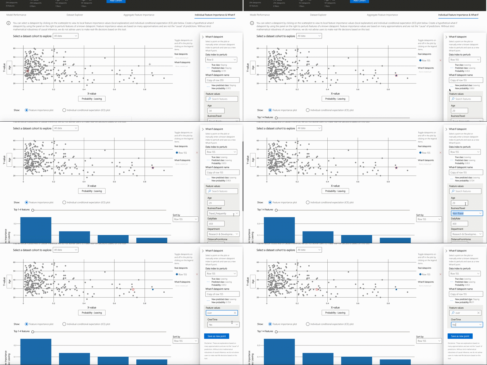
- Individual Feature Importance and What-If
Note
Click on "Open in a new tab" on the top left corner to get a better view of the dashboard in a new tab.
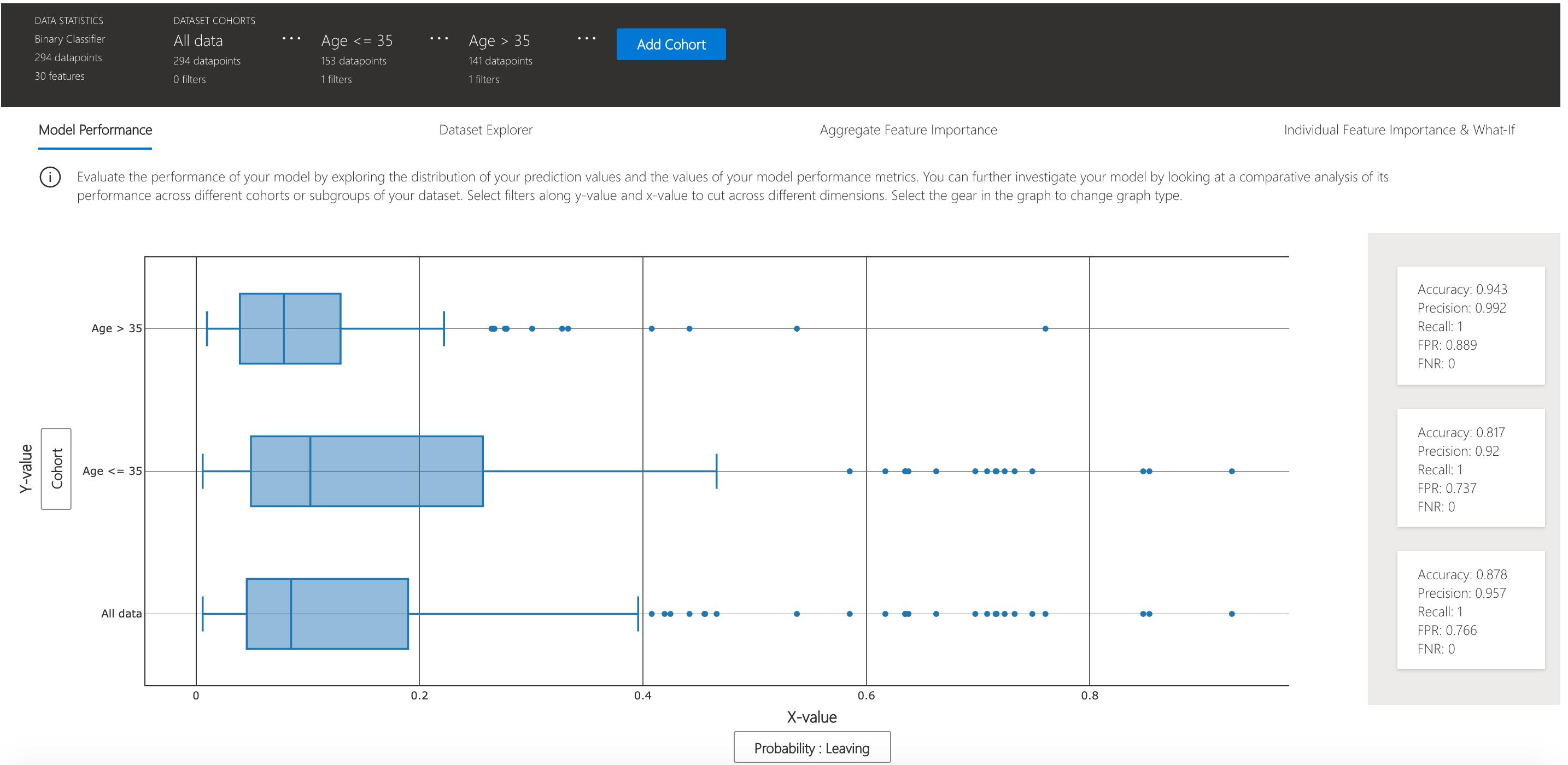
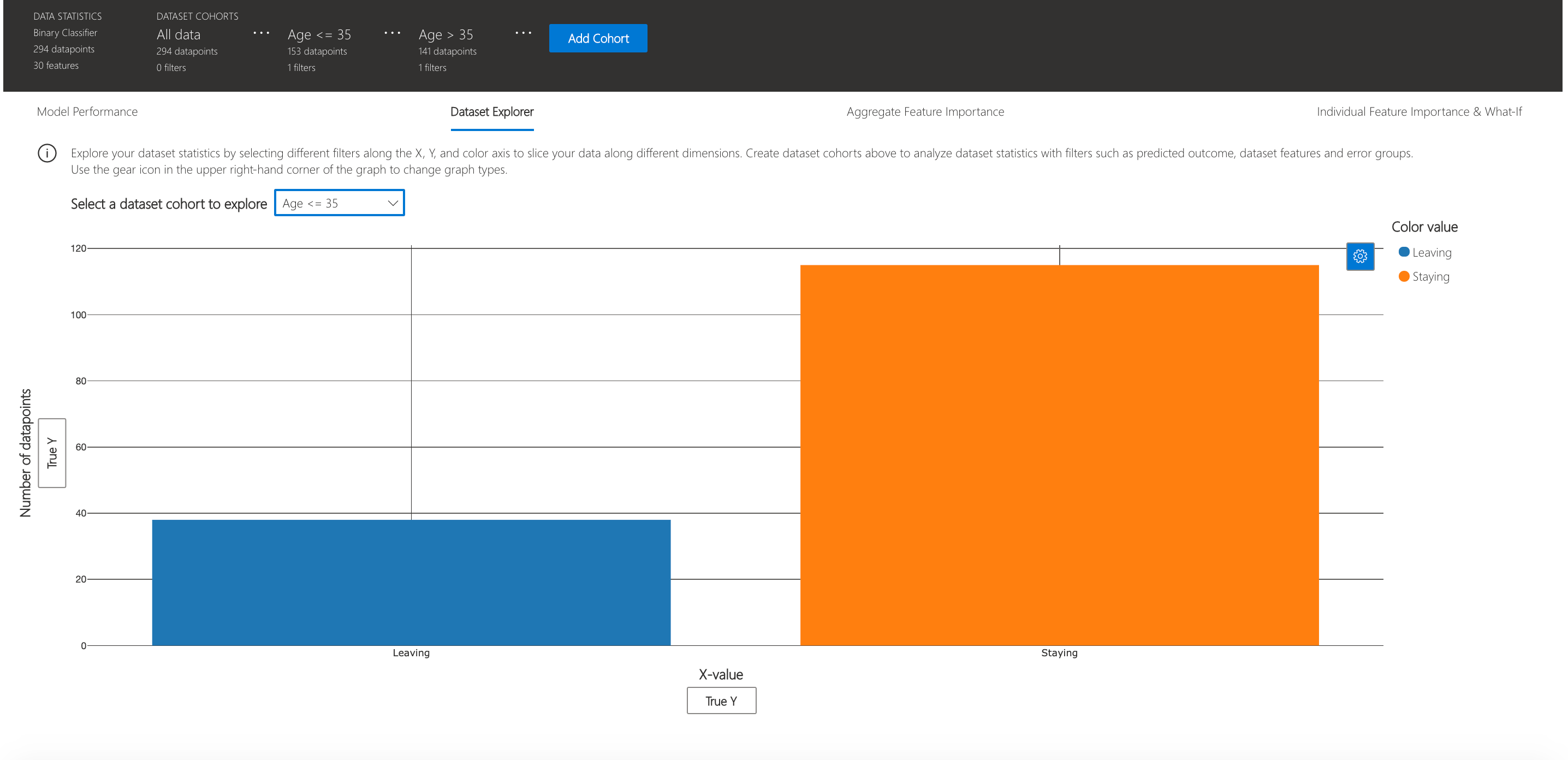
You can further create custom cohorts (subgroups of your dataset) to explore the insights across different subgroups (e.g., women vs. men). The created cohorts can contain more than one filter (e.g., age < 30 and sex = female) and will be visible from all of the four tabs. The following sections demonstrate the visualization dashboard capabilities on a classification model trained on employee attrition dataset. Besides the default cohort (including the whole dataset), there are two additional cohorts created: employees with Age <= 35 and employees with Age > 35.
This tab enables you to evaluate your model by observing its performance metrics and prediction probabilities/classes/values across different cohorts.
You can explore your dataset statistics by selecting different filters along the X, Y, and color axes of this tab to slice your data into different dimensions.
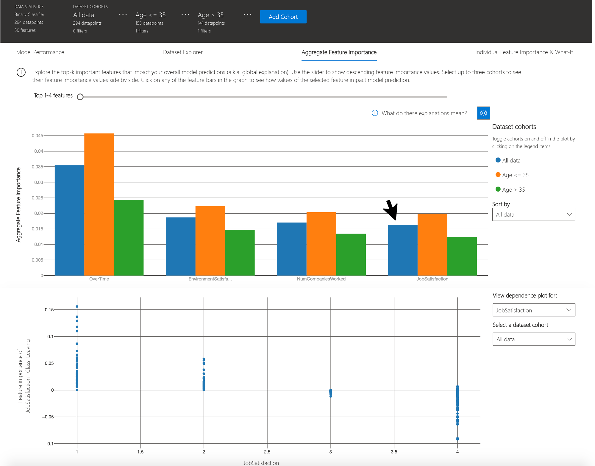
The following plots provide a global view of the trained model along with its predictions and explanations.
This view consists of two charts:
| Plot | Description |
|---|---|
| Feature Importance | Explore the top K important features that impact your overall model predictions (a.k.a. global explanation). Use the slider to show additional less important feature values. Select up to three cohorts to see their feature importance values side by side. |
| Dependence Plot | Click on any of the feature bars in the feature importance graph to see the relationship of the values of the selected feature to its corresponding feature importance values. Overall, this plot show how values of the selected feature impact model prediction. |
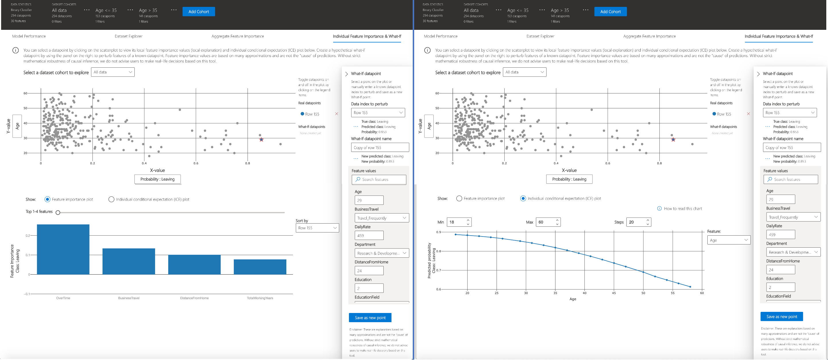
You can click on any individual data point on the scatter plot to view its local feature importance values (local explanation) and individual conditional expectation (ICE) plot below. These are the capabilities covered in this tab:
| Plot | Description |
|---|---|
| Feature Importance Plot | Shows the top K (configurable K) important features for an individual prediction. Helps illustrate the local behavior of the underlying model on a specific data point. |
| Individual Conditional Expectation (ICE) | Allows feature value changes from a minimum value to a maximum value. Helps illustrate how the data point's prediction changes when a feature changes. |
| Perturbation Exploration (what if analysis) | Allows changes to feature values of the selected data point and observe resulting changes to prediction value. You can then save your hypothetical what-if data point. |
This project welcomes contributions and suggestions. Most contributions require you to agree to the Github Developer Certificate of Origin, DCO. For details, please visit https://probot.github.io/apps/dco/.
The Developer Certificate of Origin (DCO) is a lightweight way for contributors to certify that they wrote or otherwise have the right to submit the code they are contributing to the project. Here is the full text of the DCO, reformatted for readability:
By making a contribution to this project, I certify that:
(a) The contribution was created in whole or in part by me and I have the right to submit it under the open source license indicated in the file; or
(b) The contribution is based upon previous work that, to the best of my knowledge, is covered under an appropriate open source license and I have the right under that license to submit that work with modifications, whether created in whole or in part by me, under the same open source license (unless I am permitted to submit under a different license), as indicated in the file; or
(c) The contribution was provided directly to me by some other person who certified (a), (b) or (c) and I have not modified it.
(d) I understand and agree that this project and the contribution are public and that a record of the contribution (including all personal information I submit with it, including my sign-off) is maintained indefinitely and may be redistributed consistent with this project or the open source license(s) involved.
Contributors sign-off that they adhere to these requirements by adding a Signed-off-by line to commit messages.
This is my commit message

Signed-off-by: Random J Developer <random@developer.example.org>
Git even has a -s command line option to append this automatically to your commit message:
$ git commit -s -m 'This is my commit message'
When you submit a pull request, a DCO bot will automatically determine whether you need to certify. Simply follow the instructions provided by the bot.
This project has adopted the his project has adopted the GitHub Community Guidelines.
Security issues and bugs should be reported privately, via email, to the Microsoft Security Response Center (MSRC) at secure@microsoft.com. You should receive a response within 24 hours. If for some reason you do not, please follow up via email to ensure we received your original message. Further information, including the MSRC PGP key, can be found in the Security TechCenter.


