Reliability Explorer (ReX) - command line version
ReX (Reliability Explorer) is a R toolbox for calculating reliability and mapping individual variations to facilitate the assessment of reliability and reproducibility in neuroscience and psychology. This toolbox provides two modules.
-
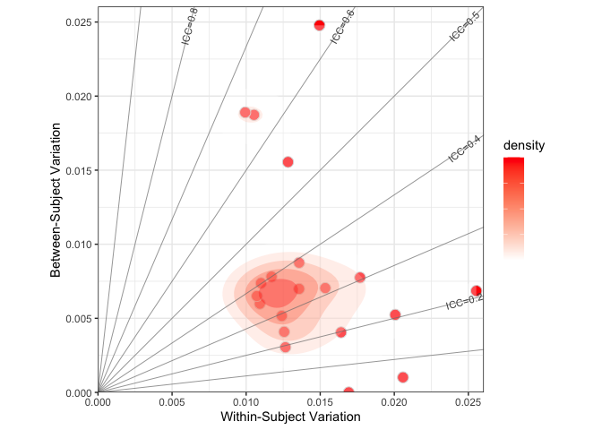
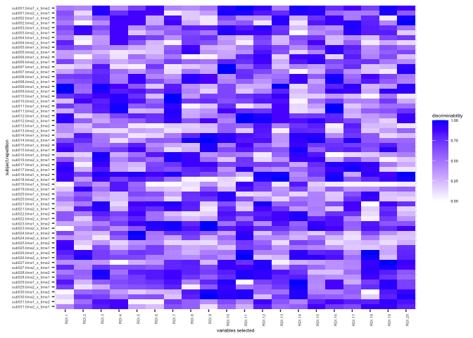
Reliability Calculation module. This module implements parametric and nonparametric methods for univariate and multivariate reliability calculation including Intraclass correlation (ICC), distance-based ICC (dbICC), Image Intraclass Correlation Coefficient (I2C2), discriminability, and identification rate (i.e. fingerprinting). The results will be presented in a two-dimensional individual variation space (x-axis: within-individual variation, y-axis: between-individual variation) to facilitate understanding of individual difference and its relation to reliability assessment. The discriminability of each observation can be used to inspect your data and results. It will help to detect (1) which variable of interest has low reliablity, (2) which observation is a potential outliers.
-
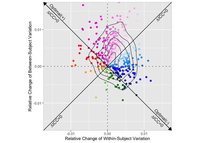
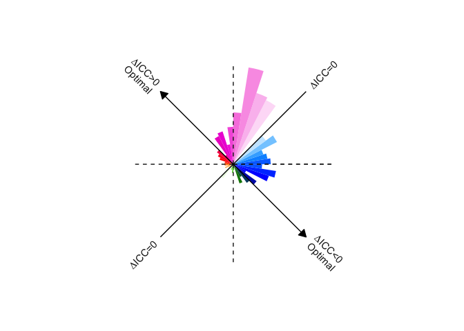
Individual Comparison module. This module provides plotting function to visualize your results in the two-dimensional individual variation space. For the paired comparison, ReX can calculate the gradient flow map provides the normalized change of the within- and between-individual variation as compared to the most efficient direction for improving ICC, which helps to guide optimization efforts for measurement of individual differences.
See Tutorials and Shiny App version: https://github.com/TingsterX/Reliability_Explorer
You can install the development version of ReX from GitHub with:
# install.packages("devtools")
devtools::install_github("TingsterX/ReX")dplyr, lme4, ggplot2, RColorBrewer, scales, stats, reshape2, colorspace, I2C2
docker pull tingsterx/rex:latest
docker run --rm \
     -v /local/path/to/your/data:/input \
     -v /local/path/to/your/output/:/output \
     tingsterx/rex:latest
The help messages and demo code are also here
docker run -it --rm --entrypoint R \
     -v /local/path/to/your/data:/input \
     -v /local/path/to/your/output/:/output \
     tingsterx/rex:latest
This is a basic example which shows you how to calculate different types of reliability
library(ReX)
# demo data is included in ReX
head(demo_brain_trt[,1:8])
#>    subID visit age gender       ROI.1       ROI.2       ROI.3       ROI.4
#> 1 sub001 time1  26      M -0.17105600  0.05934696 -0.07569620 -0.13993092
#> 2 sub001 time2  26      M -0.07177064 -0.15806658 -0.09585763  0.02516391
#> 3 sub002 time1  30      M -0.25261160  0.15716580 -0.01088339 -0.25046000
#> 4 sub002 time2  30      M -0.15065471 -0.20617760 -0.17913395 -0.28043227
#> 5 sub003 time1  38      F -0.24426076 -0.26057101 -0.39224511 -0.34416539
#> 6 sub003 time2  38      F -0.16579377 -0.23880201 -0.27823357 -0.31587505
In this example, we only illustrate 20 dependent variables from the demo data here
data <- as.matrix(demo_brain_trt[,5:24])
subID <- as.matrix(demo_brain_trt[,"subID"])
session <- as.matrix(demo_brain_trt[,"visit"])
cov <- as.matrix(demo_brain_trt[,c("age", "gender")])# Calculate the univariable Reliability: Demonstrate One-way Random Model based ICC
df_icc <- data.frame(lme_ICC_1wayR(data, subID, session, cov))
#> [1] "Running LMM for 5.00 present ..."
#> boundary (singular) fit: see help('isSingular')
head(df_icc)
#> ICC ICCk sigma2_b sigma2_w var.data error.message
#> ROI.1 0.20704401 0.34305959 0.005238936 0.02006455 0.02537167 0
#> ROI.2 0.04698971 0.08976155 0.001015134 0.02058820 0.02127059 0
#> ROI.3 0.64010940 0.78056915 0.018732651 0.01053211 0.02594836 0
#> ROI.4 0.39197004 0.56318747 0.008752628 0.01357721 0.02105680 0
#> ROI.5 0.31462057 0.47864848 0.007041670 0.01533980 0.02380350 0
#> ROI.6 0.29384289 0.45421726 0.005162441 0.01240627 0.01862917 0
# The within- and between-individual variation map
rex_plot.var.field(df_icc, size.point = 4, alpha.density = 0.3, color.point.fill = "red", color="red")# Calculate the univariable Reliability Discriminability
Discr_list <- discriminability_wraper(data, subID, session, all_discr.return=TRUE)
#> [1] 62
#> [1] 2
# Discriminability for each dependent variable
head(Discr_list$Discr)
#> discriminability
#> ROI.1 0.5565574
#> ROI.2 0.4650538
#> ROI.3 0.6341398
#> ROI.4 0.5521505
#> ROI.5 0.5879032
#> ROI.6 0.5252688
# Discriminability for each observation and dependent variable
head(Discr_list$DiscrSub[1:6,1:6])
#> subID combination ROI.1 ROI.2 ROI.3 ROI.4
#> 1 sub001 time1_x_time2 0.4666667 0.43333333 0.9500000 0.4166667
#> 2 sub001 time2_x_time1 0.6333333 0.13333333 0.9666667 0.7500000
#> 3 sub002 time1_x_time2 0.5666667 0.31666667 0.6000000 0.9000000
#> 4 sub002 time2_x_time1 0.4666667 0.01666667 0.4000000 0.8833333
#> 5 sub003 time1_x_time2 0.6666667 0.93333333 0.6500000 0.8833333
#> 6 sub003 time2_x_time1 0.5666667 0.90000000 0.5333333 0.8833333
# Inspect the Discriminability for each observation and dependent variable
rex_plot.discri_matrix(Discr_list$DiscrSub[,-c(1,2)], Discr_list$DiscrSub[,1], Discr_list$DiscrSub[,2])iRate_list <- fingerprinting_wraper(data, subID, session, method.dist = 'euclidean')
head(iRate_list$FP)
#> fingerprinting
#> ROI.1 0.03225806
#> ROI.2 0.00000000
#> ROI.3 0.00000000
#> ROI.4 0.00000000
#> ROI.5 0.00000000
#> ROI.6 0.00000000# All multivariable reliability are based on the distance matrix
Dmax <- dist(data, method = "euclidean")
# I2C2
calc_i2c2(Dmax, subID, as.matrix(session))
#> [1] 0.3311749
# dbICC
calc_dbICC(Dmax, subID)
#> $dbicc
#> [1] 0.3557867
#>
#> $var_w
#> [1] 0.2915027
#>
#> $var_b
#> [1] 0.1609914
# discriminability
calc_discriminability(Dmax, subID)
#> [1] 0.7223118
# identification rate (fingerprinting)
calc_fingerprinting(Dmax, subID)
#> [1] 0.03225806
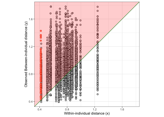
# plot the distance space (red shade: discriminated observations, red dot: identified observation)
dFM.df <- distance_field_map.df(Dmax, subID)
rex_plot.distance_field_map(dFM.df, point.size = 2)Demo data included in ReX: reliability and variation of brain connectivity preprocessed with and without global signal regression (GSR).
# 62 observations includes 31 subjects and 2 visits per subject
df_baseline <- demo_icc_noGSR
df_target <- demo_icc_GSR
df_paired <- cbind(df_baseline, df_target)
# calculate the normalized changes of variation - gradient flow
df_VarPairedComp <- icc_gradient_flow(df_target[,"sigma2_w"], df_target[,"sigma2_b"], df_baseline[,"sigma2_w"], df_baseline[,"sigma2_b"])
df_VarPairedComp$contrast <- "GSR - noGSR"
rownames(df_VarPairedComp) <- df_paired$X
head(df_VarPairedComp)
#>       delta.sigma2_w delta.sigma2_b delta.theta delta.sigma2_w_norm
#> V1_L    0.0067027234   0.0041337102   0.5526237         0.002800307
#> MST_L   0.0069396022  -0.0036147009   5.8029735         0.007812760
#> V6_L   -0.0008516454  -0.0014259651   4.1740003        -0.001146563
#> V2_L    0.0051266349  -0.0011036842   6.0711374         0.005140554
#> V3_L    0.0055806057  -0.0001105027   6.2633867         0.005539193
#> V4_L    0.0060191643  -0.0020029545   5.9619482         0.005864097
#>       delta.sigma2_b_norm delta.theta_norm    contrast
#> V1_L         0.0073601864       1.20724146 GSR - noGSR
#> MST_L        0.0004300274       0.05498619 GSR - noGSR
#> V6_L        -0.0012016940       3.95046375 GSR - noGSR
#> V2_L        -0.0010369238       6.08414181 GSR - noGSR
#> V3_L         0.0006875364       0.12349052 GSR - noGSR
#> V4_L        -0.0024196136       5.89185158 GSR - noGSR
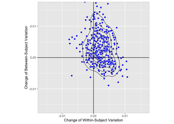
Change of the within- and between-individual variation: target (GSR) vs baseline (noGSR)
rex_plot.var.change(df_VarPairedComp)Normalized (relative) change of the within- and between-individual variation: target (GSR) vs baseline (noGSR)
rex_plot.icc.gradient.norm(df_VarPairedComp)# Hisgotram of normalized change of the variation - gradient flow: target vs baseline
rex_plot.icc.gradient.hist(df_VarPairedComp)v1.0.0 - July 10 2022
v1.0.1 - Oct 30 2022
- fix bug: If input data contains NA in Discriminability/Fingerprinting calculation (listwise delete)
- fix bug: If input data contains >2 visits per subject in Discriminability/Fingerprinting calculation
- add dbICC based within- and between-individual variation
