pip install keras-tcnKeras Temporal Convolutional Network
- Keras TCN
- TCNs exhibit longer memory than recurrent architectures with the same capacity.
- Constantly performs better than LSTM/GRU architectures on a vast range of tasks (Seq. MNIST, Adding Problem, Copy Memory, Word-level PTB...).
- Parallelism, flexible receptive field size, stable gradients, low memory requirements for training, variable length inputs...
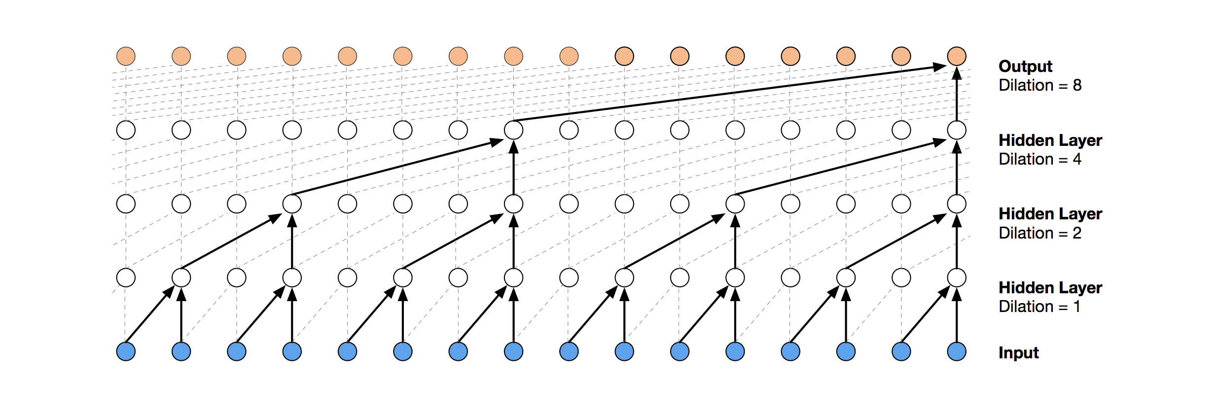 Visualization of a stack of dilated causal convolutional layers (Wavenet, 2016)
The usual way is to import the TCN layer and use it inside a Keras model. An example is provided below for a regression task (cf. tasks/ for other examples):
from tensorflow.keras.layers import Dense
from tensorflow.keras import Input, Model

from tcn import TCN, tcn_full_summary

batch_size, timesteps, input_dim = None, 20, 1


def get_x_y(size=1000):
    import numpy as np
    pos_indices = np.random.choice(size, size=int(size // 2), replace=False)
    x_train = np.zeros(shape=(size, timesteps, 1))
    y_train = np.zeros(shape=(size, 1))
    x_train[pos_indices, 0] = 1.0
    y_train[pos_indices, 0] = 1.0
    return x_train, y_train


i = Input(batch_shape=(batch_size, timesteps, input_dim))

o = TCN(return_sequences=False)(i)  # The TCN layers are here.
o = Dense(1)(o)

m = Model(inputs=[i], outputs=[o])
m.compile(optimizer='adam', loss='mse')

tcn_full_summary(m, expand_residual_blocks=False)

x, y = get_x_y()
m.fit(x, y, epochs=10, validation_split=0.2)
In the example above, TCNs can also be stacked together, like this:
o = TCN(return_sequences=True)(i)
o = TCN(return_sequences=False)(o)
A ready-to-use TCN model can be used that way (cf. tasks/ for the full code):
from tcn import compiled_tcn

model = compiled_tcn(...)
model.fit(x, y) # Keras model.TCN(nb_filters=64, kernel_size=2, nb_stacks=1, dilations=[1, 2, 4, 8, 16, 32], padding='causal', use_skip_connections=True, dropout_rate=0.0, return_sequences=True, activation='linear', kernel_initializer='he_normal', use_batch_norm=False, **kwargs)
nb_filters: Integer. The number of filters to use in the convolutional layers. Would be similar tounitsfor LSTM.kernel_size: Integer. The size of the kernel to use in each convolutional layer.dilations: List. A dilation list. Example is: [1, 2, 4, 8, 16, 32, 64].nb_stacks: Integer. The number of stacks of residual blocks to use.padding: String. The padding to use in the convolutions. 'causal' for a causal network (as in the original implementation) and 'same' for a non-causal network.use_skip_connections: Boolean. If we want to add skip connections from input to each residual block.return_sequences: Boolean. Whether to return the last output in the output sequence, or the full sequence.dropout_rate: Float between 0 and 1. Fraction of the input units to drop.activation: The activation used in the residual blocks o = activation(x + F(x)).kernel_initializer: Initializer for the kernel weights matrix (Conv1D).use_batch_norm: Whether to use batch normalization in the residual layers or not.kwargs: Any other arguments for configuring parent class Layer. For example "name=str", Name of the model. Use unique names when using multiple TCN.
3D tensor with shape (batch_size, timesteps, input_dim).
timesteps can be None. This can be useful if each sequence is of a different length: Multiple Length Sequence Example.
- if
return_sequences=True: 3D tensor with shape(batch_size, timesteps, nb_filters). - if
return_sequences=False: 2D tensor with shape(batch_size, nb_filters).
- Regression (Many to one) e.g. adding problem
- Classification (Many to many) e.g. copy memory task
- Classification (Many to one) e.g. sequential mnist task
For a Many to Many regression, a cheap fix for now is to change the number of units of the final Dense layer.
- Receptive field = nb_stacks_of_residuals_blocks * kernel_size * last_dilation.
- If a TCN has only one stack of residual blocks with a kernel size of 2 and dilations [1, 2, 4, 8], its receptive field is 2 * 1 * 8 = 16. The image below illustrates it:
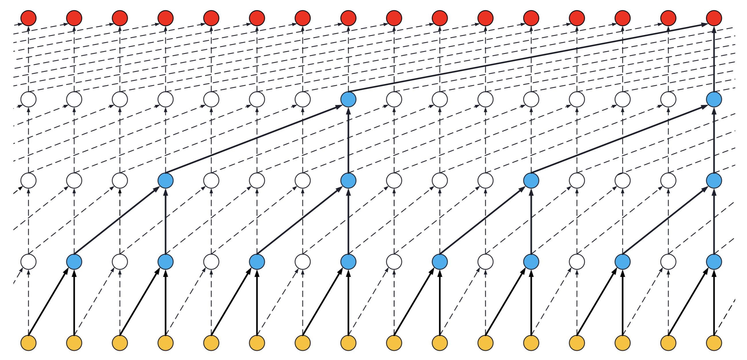 ks = 2, dilations = [1, 2, 4, 8], 1 block
- If the TCN has now 2 stacks of residual blocks, wou would get the situation below, that is, an increase in the receptive field to 32:
 ks = 2, dilations = [1, 2, 4, 8], 2 blocks
- If we increased the number of stacks to 3, the size of the receptive field would increase again, such as below:
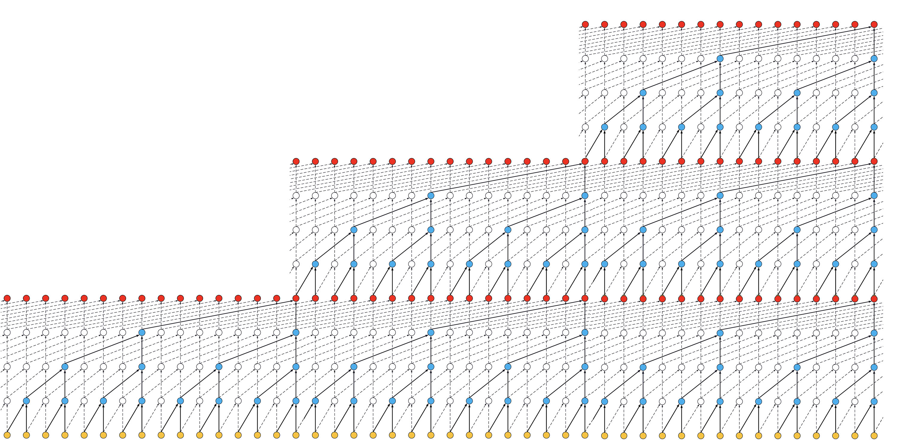 ks = 2, dilations = [1, 2, 4, 8], 3 blocks
Thanks to @alextheseal for providing such visuals.
Making the TCN architecture non-causal allows it to take the future into consideration to do its prediction as shown in the figure below.
However, it is not anymore suitable for real-time applications.
 Non-Causal TCN - ks = 3, dilations = [1, 2, 4, 8], 1 block
To use a non-causal TCN, specify padding='valid' or padding='same' when initializing the TCN layers.
Special thanks to: @qlemaire22
git clone git@github.com:philipperemy/keras-tcn.git
cd keras-tcn
virtualenv -p python3.6 venv
source venv/bin/activate
pip install -r requirements.txt # change to tensorflow if you dont have a gpu.
pip install . --upgrade # install it as a package.
Note: Only compatible with Python 3 at the moment. Should be almost compatible with python 2.
Once keras-tcn is installed as a package, you can take a glimpse of what's possible to do with TCNs. Some tasks examples are available in the repository for this purpose:
cd adding_problem/
python main.py # run adding problem task

cd copy_memory/
python main.py # run copy memory task

cd mnist_pixel/
python main.py # run sequential mnist pixel task
Reproducible results are possible on (NVIDIA) GPUs using the tensorflow-determinism library. It was tested with keras-tcn by @lingdoc and he got reproducible results.
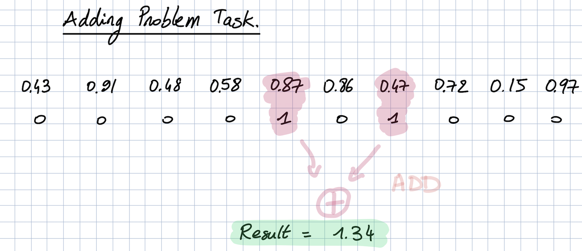
The task consists of feeding a large array of decimal numbers to the network, along with a boolean array of the same length. The objective is to sum the two decimals where the boolean array contain the two 1s.
The model takes time to learn this task. It's symbolized by a very long plateau (could take ~8 epochs on some runs).
200000/200000 [==============================] - 293s 1ms/step - loss: 0.1731 - val_loss: 0.1662
200000/200000 [==============================] - 289s 1ms/step - loss: 0.1675 - val_loss: 0.1665
200000/200000 [==============================] - 287s 1ms/step - loss: 0.1670 - val_loss: 0.1665
200000/200000 [==============================] - 288s 1ms/step - loss: 0.1668 - val_loss: 0.1669
200000/200000 [==============================] - 285s 1ms/step - loss: 0.1085 - val_loss: 0.0019
200000/200000 [==============================] - 285s 1ms/step - loss: 0.0011 - val_loss: 4.1667e-04
200000/200000 [==============================] - 282s 1ms/step - loss: 6.0470e-04 - val_loss: 6.7708e-04
200000/200000 [==============================] - 282s 1ms/step - loss: 4.3099e-04 - val_loss: 7.3898e-04
200000/200000 [==============================] - 282s 1ms/step - loss: 3.9102e-04 - val_loss: 1.8727e-04
200000/200000 [==============================] - 280s 1ms/step - loss: 3.1040e-04 - val_loss: 0.0010
200000/200000 [==============================] - 281s 1ms/step - loss: 3.1166e-04 - val_loss: 2.2333e-04
200000/200000 [==============================] - 281s 1ms/step - loss: 2.8046e-04 - val_loss: 1.5194e-04
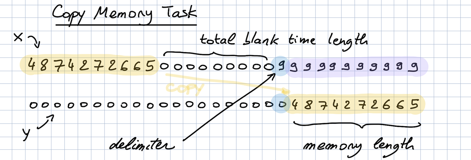
The copy memory consists of a very large array:
- At the beginning, there's the vector x of length N. This is the vector to copy.
- At the end, N+1 9s are present. The first 9 is seen as a delimiter.
- In the middle, only 0s are there.
The idea is to copy the content of the vector x to the end of the large array. The task is made sufficiently complex by increasing the number of 0s in the middle.
30000/30000 [==============================] - 30s 1ms/step - loss: 0.1174 - acc: 0.9586 - val_loss: 0.0370 - val_acc: 0.9859
30000/30000 [==============================] - 26s 874us/step - loss: 0.0367 - acc: 0.9859 - val_loss: 0.0363 - val_acc: 0.9859
30000/30000 [==============================] - 26s 852us/step - loss: 0.0361 - acc: 0.9859 - val_loss: 0.0358 - val_acc: 0.9859
30000/30000 [==============================] - 26s 872us/step - loss: 0.0355 - acc: 0.9859 - val_loss: 0.0349 - val_acc: 0.9859
30000/30000 [==============================] - 25s 850us/step - loss: 0.0339 - acc: 0.9864 - val_loss: 0.0291 - val_acc: 0.9881
30000/30000 [==============================] - 26s 856us/step - loss: 0.0235 - acc: 0.9896 - val_loss: 0.0159 - val_acc: 0.9944
30000/30000 [==============================] - 26s 872us/step - loss: 0.0169 - acc: 0.9929 - val_loss: 0.0125 - val_acc: 0.9966
The idea here is to consider MNIST images as 1-D sequences and feed them to the network. This task is particularly hard because sequences are 28*28 = 784 elements. In order to classify correctly, the network has to remember all the sequence. Usual LSTM are unable to perform well on this task.
60000/60000 [==============================] - 118s 2ms/step - loss: 0.2348 - acc: 0.9265 - val_loss: 0.1308 - val_acc: 0.9579
60000/60000 [==============================] - 116s 2ms/step - loss: 0.0973 - acc: 0.9698 - val_loss: 0.0645 - val_acc: 0.9798
[...]
60000/60000 [==============================] - 112s 2ms/step - loss: 0.0075 - acc: 0.9978 - val_loss: 0.0547 - val_acc: 0.9894
60000/60000 [==============================] - 111s 2ms/step - loss: 0.0093 - acc: 0.9968 - val_loss: 0.0585 - val_acc: 0.9895
Testing is based on Tox.
pip install tox
tox
- https://github.com/locuslab/TCN/ (TCN for Pytorch)
- https://arxiv.org/pdf/1803.01271.pdf (An Empirical Evaluation of Generic Convolutional and Recurrent Networks for Sequence Modeling)
- https://arxiv.org/pdf/1609.03499.pdf (Original Wavenet paper)
- https://github.com/Baichenjia/Tensorflow-TCN (Tensorflow Eager implementation of TCNs)
