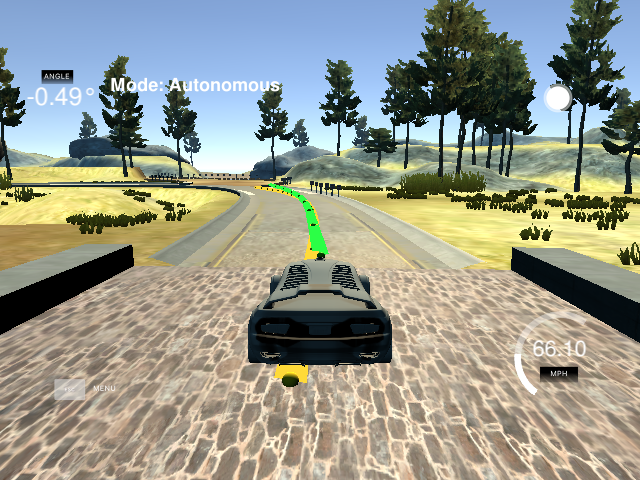
- Please see the repository from Udacity.
- Replace all the files in the folder
src.
The video was uploaded on Youtube. link The ref_v was set fixed as 70 mph.
Another video was also uploaded. link The ref_v was set as 100 mph, when abs(cte) was less than 1. ref_v was set as 50 mph, when abs(cte) was larger than 1.
            ^  y
            |
    --------|--------
    |       |       |
    |       O-------------> x           -----> velocity
    |   vehicle     |
    -----------------
rear                front
deltais the steering wheel angle. The bound is (-25, 25) degree.ais the throttle (when > 0) and brake (when < 0). The bound is (-1, 1).
xis the x coordinate of the vehicle.yis the y coordinate of the vehicle.psiis the yaw angle of the vehicle.vis the velocity in direction in front of the vehicle.cteis the cross track error at this moment.epsiis the orientation error
x = x + v * cos(psi) * dty = y + v * sin(psi) * dtpsi = psi + v / Lf * delta * dt(slightly different in the code due to the different coordinates in simulator)v = v + a * dtcte = cte + v * sin(epsi) * dt = f(x) - y + v * sin(epsi) * dtepsi = epsi + v / Lf * delta * dt = psi - psi_des + v / Lf * delta * dt(slightly different in the code)
whereby psi_des is the desired psi. f(x) is the reference line. Lf is the length between the gravity center and the front of the vehicle.
Tis the duration, in which the predictive trajectory will be calculated. This value should be large enough, but, it is not allowed to be much large.
When it is too large: firstly the trajectory would go beyond the horizon, which will make no sense; secondly, a high value can introduce error,
due to that the reference path is approximated through a polynomial.
Thus a high value of T requires that the reference path should also be accurate sufficiently, which is not possible;
thirdly the computation will even be too much.
When it is too small, the evaluation of the trajectory is not sufficient, to have a precise optimization result.
It is recommended by Udacity that T is set to be a few seconds.
Nthe number of discretization. WhenNis too high, the computation will be too much. WhenNis too small, the predicted values will be not sufficiently accurate.dtis for the discretization ofT. It should not be too large or too small. The reason is similar to above.T = N * dt
The coordinates values, which would be sent to the optimization solver, were preprocessed. The global coordinates of the waypoints would be changed into the view of the vehicle, which means the coordinates values was changed according to the position of the vehicle (x, y, psi), so that x = 0, y = 0, psi = 0.
This preprocessing would simplify the numerical calculation, such as the calculation of cte, epsi and the optimization process.
In a real car, an actuation command won't execute instantly - there will be a delay as the command propagates through the system. A realistic delay might be on the order of 100 milliseconds. This is a problem called "latency".
MPC can deal with latency easier, because this type of delay can be incorporated as dynamics into the model. For instance, instead of considering the actual current state the MPC will calculate the state after the delay (this is like "prediction") and use this state as the "current" state.
In my implementation:
- The state
x, y, psi, vafter100 mswould be calculated. - The coordinates of waypoints would be changed according to this new state (the state after 100 ms).
- Other variables would be calculated, such as
cte, epsiandcoeffs, so that the state after100 mswould be the first state to be considered.
- The cost function would be defined according to the needs. For instance, the errors were not allowed to be much high, the changing rate of the steering angle was not allowed to be much large, etc.
- The variables were the states and the actuators at each time point except the first time point.
- The equality constraints were the updates of the states.
- Udacity Self-Driving Car Nanodegree
