PM2.5 Density Prediction based on a Two-Stage Rolling Forecast Model using LightGBM

This repo is created for storing relevant programs used in my air quality prediction project.

Dataset description

Found in UCI Machine Learning Repository, the dataset is a collection of PM2.5 concentration statistics in five Chinese cities between the beginning of 2010 and the end of 2015, and we only use the dataset of Beijing (BeijingPM20100101_20151231.csv).

Attributes in the original dataset

After some data preprocessing, we classify the dataset attributes (columns) into two types:

Label columns: All these columns combined denote the time when the values are recorded.

year: Year of the record
season: 1=Spring, 2=Summer, 3=Fall, 4=Winter
month: Month of the record
day: Day of the record
hour: Hour at which the row is recorded

Value columns: PM2.5 concentration and other meteorological parameters

PM_Dongsi,PM_Dongsihuan,PM_Nongzhanguan,PM_US Post: PM2.5 Concentration measured in different stations (ug/m³)
DEWP: Celsius Dew Point
TEMP: Celsius temperature
HUMI: Humidity (%)
PRES: Air Pressure (hPa, i.e. 1 hPa=100 Pa)
precipitation: Precipitation (millimeters)
Iprec: Cumulated precipation (millimeters)
cbwd: Combined wind direction (cv refers to still wind, NE and others refer to geographic direction)
Iws: Cumulated wind speed (m/s)

Academic information

Dataset's Digital Object Identifier (DOI): doi:10.1002/2016JD024877

Citation:

Liang, X., S. Li, S. Zhang, H. Huang, and S. X. Chen (2016), PM2.5 data reliability, consistency, and air quality assessment in five Chinese cities, J. Geophys. Res. Atmos., 121, 10220-10236.

Data Preprocessing

Technical details about this section can be found in pm25_preprocessing.ipynb

Outliers removal

We discovered that this dataset contains both outliers and missing values, so we follow certain schemes to remove anomalous values and refill them with missing value imputation techniques. First, we identify any values that do not fall within a specific normal range as outliers. Then, we set these values to NAN and handle them with imputation techniques.

Missing values imputation

The original dataset contains many missing values, and more of them emerge after removing anomalies. As a result, we adopt a variety of methods to impute them: we use Next Observation Carried Backward (NOCB) to impute missing values appearing at the beginning of the records; we use Last Observation Carried Forward (LOCF) to handle missing values at the end of the records; and at last, we use linear interpolation to handle missing values that emerge in rest of the places.

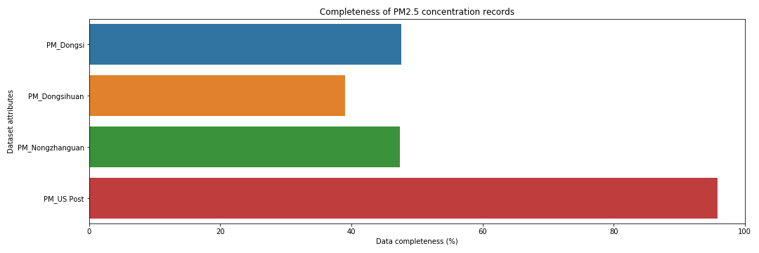
Since the dataset contains PM2.5 measured by multiple stations, we decide to impute and use the PM2.5 data measured in the U.S. Diplomatic Post because it contains the most complete PM2.5 data in compared to those in other stations.

Handling non-numerical attributes

In our dataset, not every attribute can be expressed in terms of real numbers. For instance, cbwd (Combined wind direction) is a categorical attribute and cannot be imputed using numerical methods. Hence, we only use NOCB and LOCF methods to handle missing values of these non-numerical attributes.

Following the imputation, we assign different numbers to different values of categorical features. In particular, we use the following instruction to handle cbwd attributes (in which data refers to the dataframe object of the dataset).

data["cbwd"]=data["cbwd"].map({"cv":0,"NW":1,"NE":2,"SE":3})

After data preprocessing, we begin analyzing the dataset itself.

Feature engineering

Technical details about this section can be found in pm25_features.ipynb

This section will be available in my report that will be published.

TravorLZH/pm25