This repo requires a modified version of geomstats that adds jax functionality, and a number of other modifications. This can be found here.
This repository contains the code for the paper Riemannian Score-Based Generative Modelling. This paper theoretically and practically extends score-based generative modelling (SGM) from Euclidean space to any connected and complete Riemannian manifold.
SGMs are a powerful class of generative models that exhibit remarkable empirical performance. Score-based generative modelling consists of a “noising” stage, whereby a diffusion is used to gradually add Gaussian noise to data, and a generative model, which entails a “denoising” process defined by approximating the time-reversal of the diffusion.
Simple install instructions are:
git clone https://github.com/oxcsml/score-sde.git
cd score-sde
git clone https://github.com/oxcsml/geomstats.git
virtualenv -p python3.9 venv
source venv/bin/activate
pip install -r requirements.txt
pip install -r requirements_exps.txt
GEOMSTATS_BACKEND=jax pip install -e geomstats
pip install -e .
requirements.txtcontains the core requirements for running the code in thescore_sdeandriemmanian_score_sdepackages. NOTE: you may need to alter the jax versions here to match your setup.requirements_exps.txtcontains extra dependencies needed for running our experiments, and using therun.pyfile provided for training / testing models. Also contains extra dependencies for using the job scheduling functionality of hydra.requirements_dev.txtcontains some handy development packages.
The bulk of the code for this project can be found in 3 places
- The
score_sdepackage contains code to run SDEs on Euclidean space. This code is modified from the code from the paper Score-Based Generative Modeling through Stochastic Differential Equations. - The
riemannian_score_sdepackage contains code needed to extend the code inscore_sdeto Riemannian manifolds. - An extended version of geomstats that adds
jaxsupport, and a number of other extensions.
Most of the models used in this paper can be though of as a pushforward of a simple density under some continuous-time transformation into a more complex density. In code, this is represented by a score_sde.models.flow.PushForward, containing a base distribution, and in the simplest case, a time dependent vector field that defines the flow of the density through time.
A Continuous Normalizing Flow (CNF) [score_sde.models.flow.PushForward]
samples from the pushforward distribution by evolving samples from the base
measure under the action of the vector field. The log-likelihood is computed by
adding the integral of the divergence of the vector field along the sample path
to the log-likelihood of the point under the base measure. Models are trained by
optimising this log-likelihood of the training data.
Moser flows [score_sde.models.flow.MoserFlow] alleviate the expensive
likelihood computation in training using an alternative, cheaper, method of
computing the likelihood. This unfortunately requires a condition on the
pushforward vector field, which is enforced by a regularisation term in the
loss. As a result the cheaper likelihood computation unreliable, and the
sampling must still be done with expensive ODE solutions.
Score-based Generative Models (SGMs) [score_sde.models.flow.SDEPushForward]
instead consider a pushforward defined by the time-reversal of a noising
Stochastic Differential Equation (SDE). Instead of relying on likelihood based
training, these models are trained using score matching. The likelihood is
computed by converting the SDE to the corresponding likelihood ODE. While
identical in nature to the likelihood ODE of CNFs/Moser flows, these are
typically easier to solve computationally due the learned vector fields
being less stiff.
Other core pieces of code include:
score_sde/models/transform.pywhich defines transforms between manifolds and Euclidean space, designed to allow for pushing a Euclidean density onto a manifold.score_sde/models/vector_field.pywhich contains various parametrisations of vector fields needed for defining the score functions / vector fieldsscore_sde/sde.pywhich defines various SDEsscore_sde/losses.pywhich contains all the loss functions usedscore_sde/sampling.pywhich provides methods for sampling SDEsscore_sde/ode.pywhich provides methods for solving ODEs
and their counterparts in riemannian_score_sde.
Models are decomposed in three blocks:
- a
basedistribution, withz ~ base(a 'prior') - a learnable diffeomorphic
flow: z -> y(the flexible component of the model, potentially stochastic as for SGMs) - a
transformmapy -> x ∈ M(if the model is not defined on the manifold and needs to be 'projected', else the model is Riemannian andtransform=Id) Thus, the generative models are defined asz -> y -> x.
Experiment configuration is handled by hydra, a highly flexible yaml based configuration package. Base configs can be found in config, and parameters are overridden in the command line. Sweeps over parameters can also be managed with a single command.
Jobs scheduled on a cluster using a number of different plugins. We use Slurm, and configs for this can be found in config/server (note these are reasonably general but have some setup-specific parts). Other systems can easily be substituted by creating a new server configuration.
The main training and testing script can be found in run.py, and is dispatched by running python main.py [OPTIONs].
By default we log to CSV files and to Weights and biases. To use weights and biases, you will need to have an appropriate WANDB_API_KEY set in your environment, and to modify the entity and project entries in the config/logger/wandb.yaml file. The top level local logging directory can be set via the logs_dir variable.
To run a toy experiment on the sphere run:
python main.py experiment=s2_toy
This should validate that the code is installed correctly and the RSGM models are training properly.
We run experiments on 4 natural disaster experiments against a number of baselines.
| Volcano | Earthquake | Flood | Fire | |
|---|---|---|---|---|
| Mixture of Kent | -0.80 ± 0.47 | 0.33 ± 0.05 | 0.73 ± 0.07 | 1.18 ± 0.06 |
| Riemannian CNF | * -6.05 ± 0.61 | 0.14 ± 0.23 | 1.11 ± 0.19 | * -0.80 ± 0.54 |
| Moser Flow | -4.21 ± 0.17 | * -0.16 ± 0.06 | * 0.57 ± 0.10 | * -1.28 ± 0.05 |
| Stereographic Score-Based (ours) | @ -3.80 ± 0.27 | * -0.19 ± 0.05 | 0.59 ± 0.07 | * -1.28 ± 0.12 |
| Riemannian Score-Based (ours) | -4.92 ± 0.25 | * -0.19 ± 0.07 | * 0.48 ± 0.09 | * -1.33 ± 0.06 |
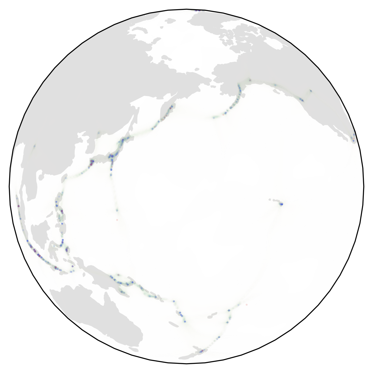
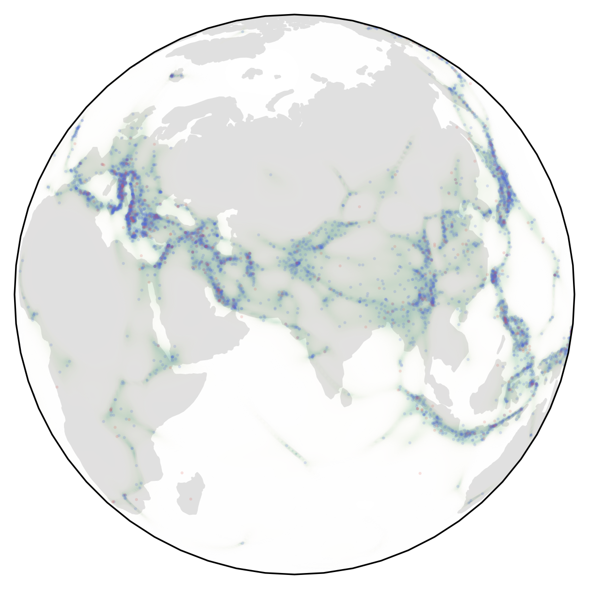
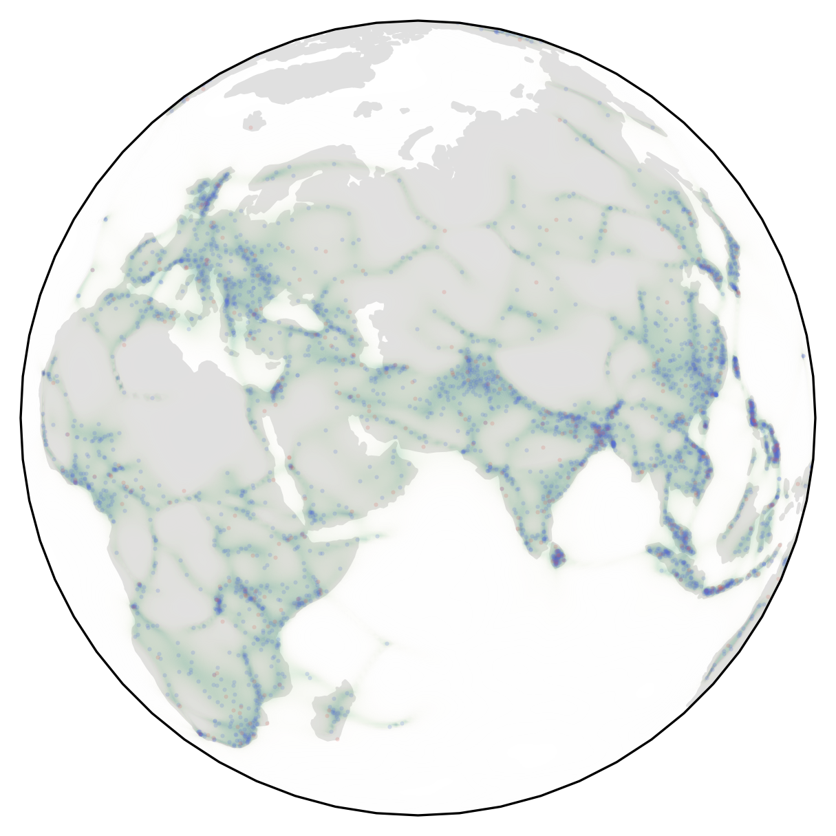
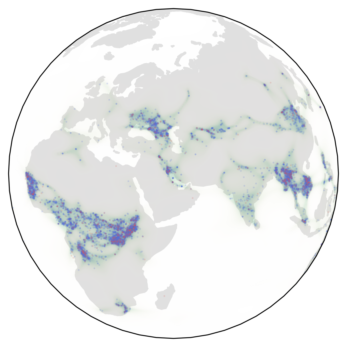
Examples of densities learned by RSGMs on the datasets:
| Volcano | Earthquake | Flood | Fire |
|---|---|---|---|
 |
 |
 |
 |
To run the full sweeps over parameters used in the paper run:
RSGM ISM loss:
python main.py -m \
    experiment=volcanoe,earthquake,fire,flood \
    model=rsgm \
    generator=div_free,ambient \
    loss=ism \
    flow.N=20,50,200 \
    flow.beta_0=0.001 \
    flow.beta_f=2,3,5 \
    steps=300000,600000 \
    seed=0,1,2,3,4
RSGM DSM loss:
python main.py -m \
    experiment=volcanoe,earthquake,fire,flood \
    model=rsgm \
    generator=div_free,ambient \
    loss=dsm0 \
    loss.thresh=0.0,0.2,0.3,0.5,0.8,1.0 \
    loss.n_max=-1,0,1,3,5,10,50 \
    flow.beta_0=0.001 \
    flow.beta_f=2,3,5 \
    seed=0,1,2,3,4
Stereo RSGMs:
python main.py -m \
    experiment=volcanoe,earthquake,fire,flood \
    model=stereo_sgm \
    generator=ambient \
    loss=ism \
    flow.beta_0=0.001 \
    flow.beta_f=4,6,8 \
    seed=0,1,2,3,4
Moser flows:
python main.py -m \
    experiment=volcanoe,earthquake,fire,flood \
    model=moser \
    loss.hutchinson_type=None \
    loss.K=20000 \
    loss.alpha_m=100 \
    seed=0,1,2,3,4
CNF:
python main.py -m \
    experiment=volcanoe,earthquake,fire,flood \
    model=cnf \
    generator=div_free,ambient \
    steps=100000 \
    flow.hutchinson_type=None \
    optim.learning_rate=1e-4 \
    seed=0,1,2,3,4
Mixture of Kent
python scripts/kent/run_kent.py -m seed=1,2,3,4,5 dataset=fire,flood,quakes_all,volerup n_components=5,10,15,20,25 iterations=50,100,150

python
To demonstrate the scaling of our method to high dimension manifolds we train RSGMs on products of circles to give high dimension toruses. We compare to the performance of Moser flows, the next most scalable method.
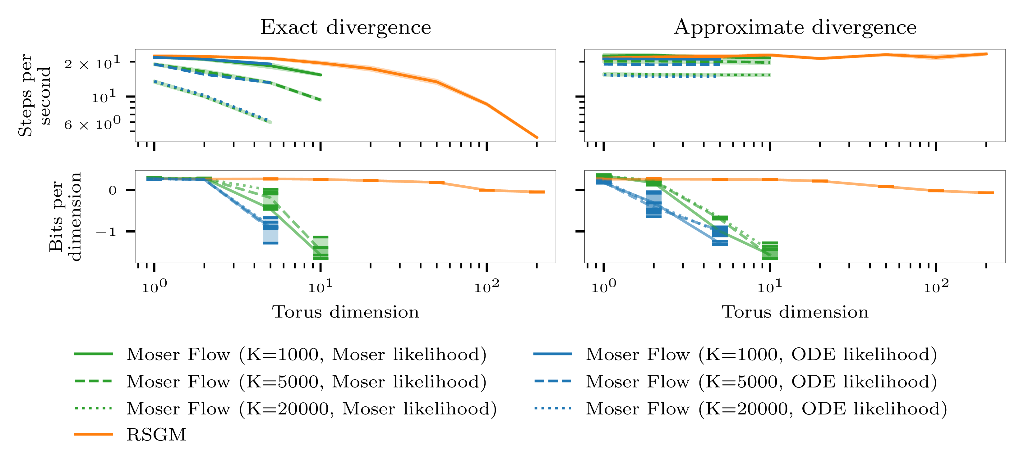
The commands to run the experiments shown in the plots are:
RSGMs:
python main.py -m \
    experiment=tn \
    n=1,2,5,10,20,50,100,200 \
    architecture.hidden_shapes=[512,512,512] \
    loss=ism,ssm \
    seed=0,1,2
Moser flows:
python main.py -m \
    experiment=tn \
    n=1,2,5,10,20,50,100,200 \
    model=moser \
    loss.hutchinson_type=None,Rademacher \
    loss.K=1000,5000,20000 \
    loss.alpha_m=1 \
    architecture.hidden_shapes=[512,512,512] \
    seed=0,1,2
To demonstrate that RSGMs can handle Lie groups as well, we train RSGMs and Moser flows on mixtures of wrapped normal distributions on
| Method | N=16, log-likelihood | N=16, NFE | N=32, log-likelihood | N=32, NFE | N=64, log-likelihood | N=64, NFE |
|---|---|---|---|---|---|---|
| Moser Flow | 0.85 ± 0.03 | 2.3 ± 0.5 | 0.17 ± 0.03 | 2.3 ± 0.9 | * -0.49 ± 0.02 | 7.3 ± 1.4 |
| Exp-wrapped SGM | * 0.87 ± 0.04 | 0.5 ± 0.1 | 0.16 ± 0.03 | 0.5 ± 0.0 | -0.58 ± 0.04 | 0.5 ± 0.0 |
| RSGM | * 0.89 ± 0.03 | * 0.1 ± 0.0 | * 0.20 ± 0.03 | * 0.1 ± 0.0 | * -0.49 ± 0.02 | * 0.1 ± 0.0 |
RSGMs
python main.py -m \
    experiment=so3 \
    model=rsgm \
    dataset.K=16,32,64 \
    steps=100000 \
    loss=dsmv \
    generator=lie_algebra \
    optim.learning_rate=5e-4,2e-4 \
    flow.beta_f=2,4,6,8,10 \
    seed=0,1,2,3,4
Exp RSGMs
python main.py -m \
    experiment=so3 \
    model=tanhexp_sgm \
    dataset.K=16,32,64 \
    steps=100000 \
    optim.learning_rate=5e-4,2e-4 \
    flow.beta_f=2,4,6,8,10 \
    seed=0,1,2,3,4
Moser flows
python main.py -m \
    experiment=so3 \
    model=moser \
    dataset.K=16,32,64 \
    steps=100000 \
    optim.learning_rate=5e-4,2e-4 \
    loss.K=1000,10000 \
    loss.alpha_m=1,10,100 \
    seed=0,1,2,3,4
So as to show that RSGMs is also suited for non-compact manifolds, we train RSGMs and an exponential map wrapped SGM baseline on mixtures of wrapped normal distributions on experiment=poincare.
RSGMs
python main.py -m \
    experiment=hyperboloid \
    model=rsgm \
    steps=100000 \
    seed=0,1,2,3,4
Exp RSGMs
python main.py -m \
    experiment=hyperboloid \
    model=exp_sgm \
    loss=dsm0 \
    generator=canonical \
    flow=vp \
    steps=100000 \
    seed=0,1,2,3,4