hystReet

Introduction

hystreet is a company collecting pedestrains in german cities. After registering you can download the data for free from 19 cities.

Installation

Until now the package is not on CRAN but you can download it via GitHub with the following command:

if (!require("devtools"))
  install.packages("devtools")
devtools::install_github("JohannesFriedrich/hystReet")

API Keys

To use this package, you will first need to get your hystreet API key. To do so, go to this link: https://hystreet.com/

Now you have three options:

Once you have your key, save it as an environment variable for the current session by running the following:

Sys.setenv(HYSTREET_API_TOKEN = "PASTE YOUR API TOKEN HERE")

Alternatively, you can set it permanently with the help of usethis::edit_r_environ() by adding the line to your .Renviron:

HYSTREET_API_TOKEN = PASTE YOUR API TOKEN HERE

If you don’t want to save it here, you can input it in each function using the API_token parameter.

Usage

Function name	Description	Example
get_hystreet_stats()	request common statistics about the hystreet project	get_hystreet_stats()
get_hystreet_locations()	request all qvailable locations	get_hystreet_locations()
get_hystreet_station_data()	request data from a stations	get_hystreet_station_data(71)
set_hystreet_token()	set your API token	set_hystreet_token(123456789)

Load some statistics

The function ‘get_hystreet_stats()’ summarises the number of available stations and the sum of all counted pedestrians.

library(hystReet)
## Loading required package: httr
## Loading required package: jsonlite
## 
## Attaching package: 'jsonlite'
## The following object is masked from 'package:purrr':
## 
##     flatten

stats <- get_hystreet_stats()

stats

stations	counts
55	352970219

Request all stations

The function ‘get_hystreet_locations()’ requests all available stations of the project.

locations <- get_hystreet_locations()

locations

id	name	city
53	Schadowstraße (West)	Düsseldorf
114	Herrenteichsstraße (Ost)	Osnabrück
94	Kurfürstendamm Südseite (Ost)	Berlin
103	Schuchardstraße	Darmstadt
108	Große Straße (Mitte)	Osnabrück
68	Petersstraße	Leipzig
95	Planken (Mitte)	Mannheim
107	Krahnstraße (Süd)	Osnabrück
54	Schadowstraße (Ost)	Düsseldorf
109	Krahnstraße (Mitte, Altstadt)	Osnabrück

Request data from a specific station

The (properly) most interesting function is ‘get_hystreet_station_data()’. With the hystreetID it is possible to request a specific station. By default, all the data from the current day are received. With the ‘query’ argument it is possible to set the received data more precise: * from: datetime of earliest measurement (default: today 00:00:00:): e.g. “10-01-2018 12:00:00” or “2018-10-01” * to : datetime of latest measurement (default: today 23:59:59): e.g. “12-01-2018 12:00:00” or “2018-12-01” * resoution: Resultion for the measurement grouping (default: hour): “day”, “hour”, “month”, “week”

data <- get_hystreet_station_data(
  hystreetId = 71, 
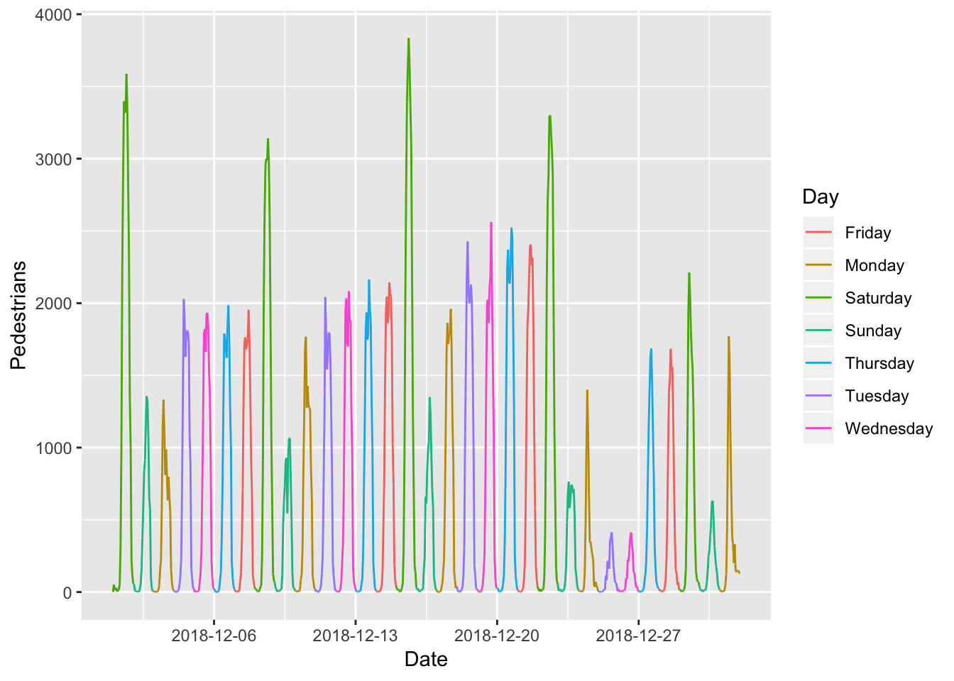
  query = list(from = "01-12-2018", to = "31-12-2018", resolution = "day"))

Some ideas to visualise the data

Let´s see if we can see the most frequent days before christmas … I think it could be saturday ;-). Also nice to see the 24th and 25th of December … holidays in Germany :-).

data <- get_hystreet_station_data(
    hystreetId = 71, 
    query = list(from = "01-12-2018", to = "01-01-2019"))

ggplot(data$measurements, aes(x = timestamp, y = pedestrians_count, colour = weekdays(timestamp))) +
  geom_path(group = 1) +
  scale_x_datetime(date_breaks = "7 days") +
  labs(x = "Date",
       y = "Pedestrians",
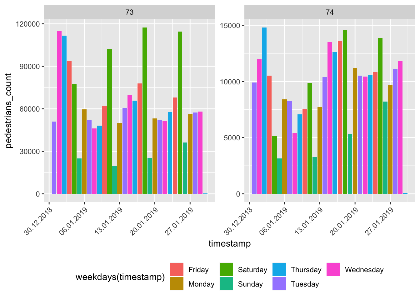
       colour = "Day")

Now let´s compare different stations:

Load the data

data_73 <- get_hystreet_station_data(
    hystreetId = 73, 
    query = list(from = "01-01-2019", to = "31-01-2019", resolution = "day"))$measurements %>% 
  select(1:2) %>% 
  mutate(station = 73)

data_74 <- get_hystreet_station_data(
    hystreetId = 74, 
    query = list(from = "01-01-2019", to = "31-01-2019", resolution = "day"))$measurements %>% 
    select(1:2) %>% 
  mutate(station = 74)

data <- bind_rows(data_73, data_74)

ggplot(data, aes(x = timestamp, y = pedestrians_count, fill = weekdays(timestamp))) +
  geom_bar(stat = "identity") +
  scale_x_datetime(labels = date_format("%d.%m.%Y")) +
  facet_wrap(~station, scales = "free_y") +
  theme(legend.position = "bottom",
        axis.text.x = element_text(angle = 45, hjust = 1))

Now a little bit of big data analysis. Let´s find the station with the highest pedestrians per day ratio:

hystreet_ids <- get_hystreet_locations()

all_data <- lapply(hystreet_ids[,"id"], function(x){
  temp <- get_hystreet_station_data(
    hystreetId = x)
  
  
    lifetime_count <- temp$statistics$lifetime_count
    days_counted <- as.numeric(temp$metadata$latest_measurement_at  - temp$metadata$earliest_measurement_at)
    
    return(data.frame(
      id = x,
      station = paste0(temp$city, " (",temp$name,")"),
      ratio = lifetime_count/days_counted))
  
})

ratio <- bind_rows(all_data)

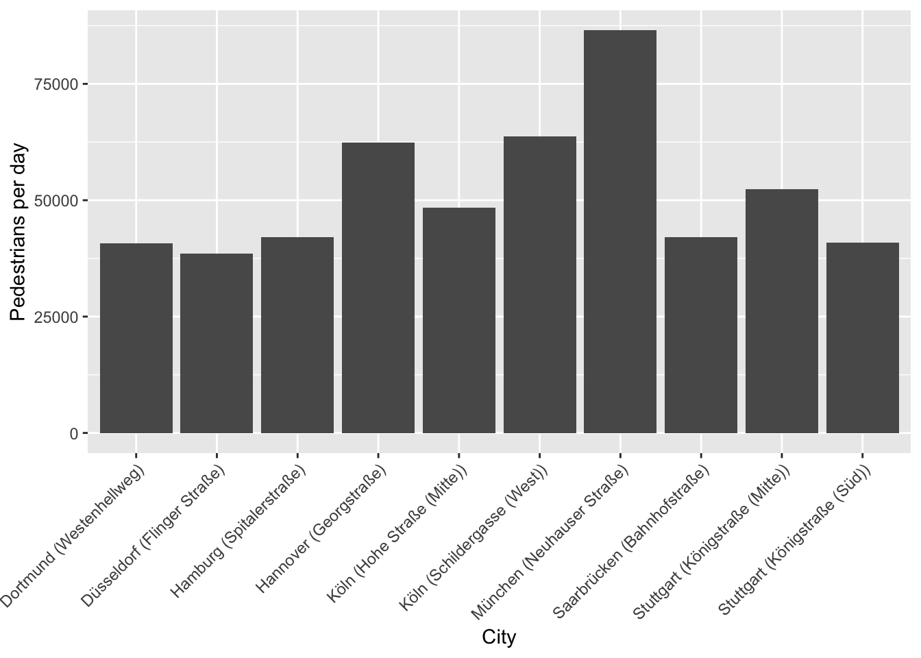
What stations have the highest ratio?

ratio %>% 
  top_n(5, ratio) %>% 
  arrange(desc(ratio))
##   id                         station    ratio
## 1 73      München (Neuhauser Straße) 86538.62
## 2 47     Köln (Schildergasse (West)) 63698.54
## 3 63          Hannover (Georgstraße) 62319.37
## 4 77 Stuttgart (Königstraße (Mitte)) 52406.47
## 5 48      Köln (Hohe Straße (Mitte)) 48382.38

Now let´s visualise the top 10 cities:

ggplot(ratio %>% 
         top_n(10,ratio), aes(station, ratio)) +
  geom_bar(stat = "identity") +
  labs(x = "City",
       y = "Pedestrians per day") + 
    theme(legend.position = "bottom",
        axis.text.x = element_text(angle = 45, hjust = 1))

Uepsilon/hystReet