This tutorial will walk through the creation and execution of a simple workflow in the Automated Service Builder (ASB), which can serve as a starting template for future workflows.
The ASB interface is built around the concept of processes and workflows, just like building a Lego set. A process can be viewed as a sort of "unit of work", a building block that has inputs/outputs and does an elementary part of the job. Each process runs in it's own docker container. A workflow is a collection of processes interconnected by their inputs and outputs, which then can be executed on the uderlying cluster.
In this example we will develop a workflow for calculating the maximum normalized difference vegetation index (NDVI). The formula for NDVI is (B8-B4)/(B8+B4), where the input bands are B4: red and B8: near-infrared part of the reflectance spectrum. Source data will be queried from VITO's Terrascope catalog by specifying vector representation of the area of interest, start/end dates and collection. We will use the Sentinel-2 L2A collection, which is divided into so-called tiles and taken dates. Hence the catalog will return a list of string pairs (B4 and B8) overlapping with our area of interest. NDVI will be computed computed at every pixel in the area of interest in a parallel fashion by processing each image pairs independently. Finally, the max NDVI image is obtained by taking the pixel-level maximum over the time period.
Please read the following parts of the documentation first:
- nomenclature: https://mep-wps.vgt.vito.be/docs/user/index.html#definitions-and-acronyms
- how to manage processes: https://mep-wps.vgt.vito.be/docs/user/index.html#processes-management
- how to manage workflows: https://mep-wps.vgt.vito.be/docs/user/index.html#workflows-management
And at least basic knowledge of Python language, since the codes used in this tutorial are written in Python.
In terms of splitting the work into units, the straightforward approach is to first query the sources, then compute NDVI in a distributed fashion and finally combine the parts together using maximum function. Within the ASB interface this would require five processes:
- Product query: obtains the list of the corresponding B4 and B8 image pairs
- Dynamic list splitter: parallelizes the work based on the query results and launches the NDVI calculators
- NDVI calculator: computes NDVI over an image pair
- Joiner: waits for all NDVI calculators to finish
- Collect_and_max: combines the outputs of the NDVI calculators
The advantage of the process/workflow system is the reusability of the processes in many different workflows. In fact 3 out of the 5 processes are readily available: product query, dynamic list splitter and the joiner processes are alreadz provided on the platform and will be reused.
Once we are done, we will combine those processes into a workflow and provide default inputs where it makes sense.
Finally, we execute the workflow to perform an actual calculation.
Login to the portal: https://mep-wps.vgt.vito.be.
As mentioned, one does not have to implement the search, rather reuse the query_product process developed by VITO. It can be used to search in the Terrascope database terrascope.be. Given the area of interest in WKT string, the date range, collection id and band names: returns the list of file names (where those are on the file system). These are the individual images that overlap with the area of interest within the date range.
We will use the following inputs:
- collection: urn:eop:VITO:TERRASCOPE_S2_TOC_V2 (Sentinel2 L2A images mirrored by Terrascope)
- date range: {"start":"2018-06-25T00:00:00", "end":"2018-06-30T00:00:00"} (JSON string covering just a few days)
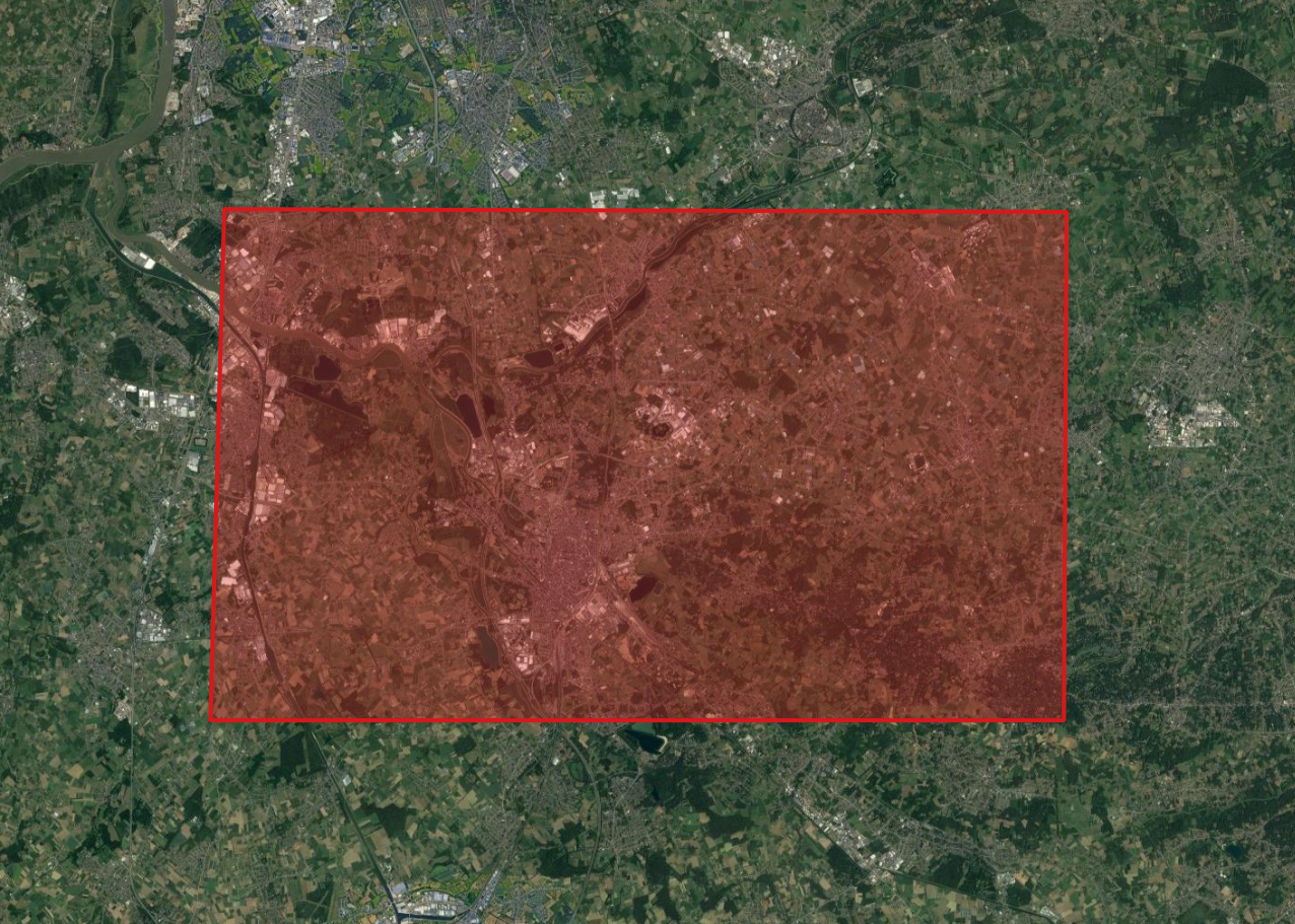
- WKT: POLYGON((4.665785 51.110600, 4.350147 51.111254, 4.344939 50.990762, 4.664744 50.990762, 4.665785 51.110600)) (small area around the Belgian city called Mechelen)
- bands: ["B04","B08"] (red and NIR bands as alread mentioned before)
The straightforward approach for the query would be to return an array JSON-ized arrays (for B4 and B8), something similar to:
[
  '["/path/to/data/S2B_20180605T105029_31UFS_TOC-B04_10M_V200.tif","/path/to/data/S2B_20180605T105029_31UFS_TOC-B08_10M_V200.tif"]',
  ...
]
Unfortunately, due to the current limitation on the length of the strings in the list imposed by the splitter, the strings have to be encoded as follows:
/path/to/data/S2B_20180605T105029_31UFS_TOC-B0+4_10M_V200.tif+8_10M_V200.tif
This string has to be split at '+' characters and the first entry is the common prefix of the rest of the array. This represents the same list of the two files as above:
/path/to/data/S2B_20180605T105029_31UFS_TOC-B04_10M_V200.tif
/path/to/data/S2B_20180605T105029_31UFS_TOC-B08_10M_V200.tif
This is also a builtin process that takes an array of strings as json. It splits up the array and indepenently launches instances of the following process in the chain. Note that the splitter is a smart process in terms of resource management: for example if 10 cpus available and each process is using 2, but the split yields to 50 processes: the splitter ensures that at a time 5 processes will be running concurrently.
This process has to be developed since it contains our 'business logic'. Let's implement it in the following fashion:
- load B4 and B8 into xarrays
- using the area of interest WKT, restrict the calculation to the bounding box
- compute NDVI
- save the resulting part into a temporary file
The main source code of any process is called process_wrapper.py, this is a Python script with a special layout that is parsed and understood by ASB.
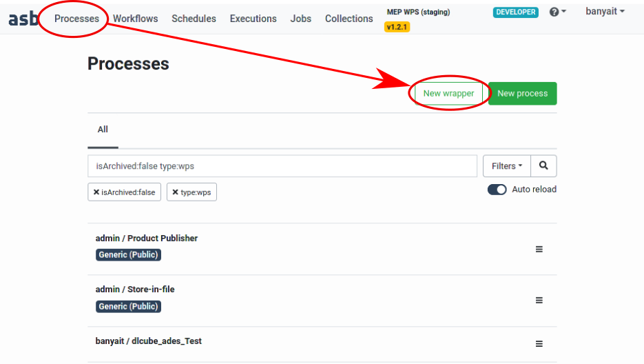
ASB provides a convenient way to generate a template, go to Processes -> New wrapper:
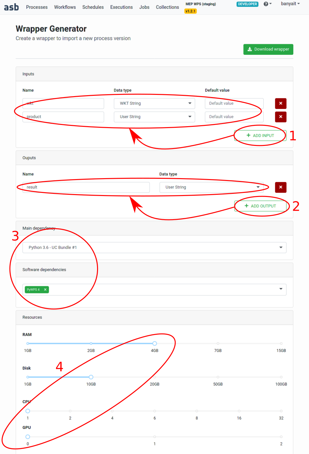
Then setup the inputs (1), outputs (2), select the dependencies (3) and resources (4) as shown:
Click on Download and save the file at a suitable location. This produces an empty wrapper to start with. Because we are going to save the results in NetCDF format, we will need an extra dependency that is not yet in the PyWPS4 software group. Next to the wrapper, save a file called requirements.txt. This file should have a single line: h5netcdf.
Open the file in your favorite editor and copy-paste the body between the two logger calls 'starting' and 'finished'. The complete contents should look like as follows:
#!/usr/bin/python

import logging
import shapely.wkt
import pyproj
import xarray
from shapely.ops import transform
import uuid
from pathlib import Path
import numpy

# --------------------------------------------------------------------------------------
# Save this code in file "process_wrapper.py" and adapt as indicated in inline comments.
#
# Notes:
#  - This is a Python 3 script.
#  - The inputs will be given values by name, thus their order has no importance ...
#  - ... except that the inputs with a default value must be listed last.
#  - Parameter names are automatically converted into valid Python variable names.
#  - Any empty line or line starting with a '#' character will be ignored.
# --------------------------------------------------------------------------------------


logger = logging.getLogger(__name__)
logging.basicConfig(level=logging.INFO)

def execute(out_dir, wkt, product):
    """
    Inputs:
    wkt -- wkt -- 92/WKT String
    product -- product -- 45/User String

    Outputs:
    result -- result -- 45/User String

    Main Dependency:
    mep-wps/uc-bundle-1

    Software Dependencies:
    pywps-4

    Processing Resources:
    ram -- 4
    disk -- 10
    cpu -- 1
    gpu -- 0
    """

    # ----------------------------------------------------------------------------------
    # Insert your own code below.
    # The files generated by your code must be stored in the "out_dir" folder.
    # Only the content of that folder is persisted in the datastore.
    # Give appropriate values to the output parameters. These will be passed to the next
    # process(es) following the workflow connections.
    # ----------------------------------------------------------------------------------

    logger.info("Starting...")

    # extract file names of the required bands
    pl=product.split("+")
    prodB4=pl[0]+[i for i in pl[1:] if "B04" in pl[0]+i][0]
    prodB8=pl[0]+[i for i in pl[1:] if "B08" in pl[0]+i][0]
    logger.info("Band B04: "+prodB4)
    logger.info("Band B08: "+prodB8)

    # open the files
    B4i=xarray.open_rasterio(prodB4)
    B8i=xarray.open_rasterio(prodB8)

    # convert area of interest into the desired coordinate system
    geom=shapely.wkt.loads(wkt)
    wgs84 = pyproj.CRS('EPSG:4326')
    gproj = pyproj.Transformer.from_crs(wgs84, B4i.crs, always_xy=True).transform
    geom = transform(gproj, geom)
    #geom=shapely.affinity.translate(geom, 120000.)
    bbox=geom.bounds

    # select part inside bbox
    B4=B4i.where((B4i.x>=bbox[0]) & (B4i.x<=bbox[2]) & (B4i.y>=bbox[1]) & (B4i.y<=bbox[3]),drop=True)
    B8=B8i.where((B8i.x>=bbox[0]) & (B8i.x<=bbox[2]) & (B8i.y>=bbox[1]) & (B8i.y<=bbox[3]),drop=True)

    # convert to floating point
    B4=B4.astype(numpy.float64)
    B8=B8.astype(numpy.float64)
    for indv in B4i.attrs.get('nodatavals',[]):
        B4=B4.where(B4!=indv, drop=True)
    for indv in B8i.attrs.get('nodatavals',[]):
        B8=B8.where(B8!=indv, drop=True)

    if B4.size>0 and B8.size>0:

        # compute NDVI
        NDVI=(B8-B4)/(B8+B4)

        # cosmetics in order for being able to save to netcdf
        NDVI.attrs['crs']=B4i.attrs['crs']
        NDVI=NDVI.assign_coords({'band':["NDVI"]})

        # Save to file
        outFile=str(Path(out_dir,"part_"+uuid.uuid4().hex))
        result=NDVI.to_dataset('band')
        result.to_netcdf(outFile, engine='h5netcdf')

        logger.info("Saved to: "+outFile)

    else:

        outFile="<EMPTY>"
        logger.info("This part is empty, skipping.")


    logger.info("Finished...")

    # ----------------------------------------------------------------------------------
    # The wrapper must return a dictionary that contains the output parameter values.
    # ----------------------------------------------------------------------------------
    return {
        "result": outFile
    }
Let's go through the details and explain what each line does:
This was generated as part of the template. When ASB executes this process, it looks for the function called execute(...). The docstring serves as metadata to define the inputs, outputs, and the resources the docker image should have. The execute function's inputs and outputs (which returns a dictionary of strings) should be in sync with this metadata. The only input parameter not listed is out_dir: this is a path to a scratch space that will be preserved between processes.
All inputs and outputs are strings, regardless of metadata types.
def execute(out_dir, wkt, product):
    """
    Inputs:
    wkt -- wkt -- 92/WKT String
    product -- product -- 45/User String

    Outputs:
    result -- result -- 45/User String

    Main Dependency:
    mep-wps/uc-bundle-1

    Software Dependencies:
    pywps-4

    Processing Resources:
    ram -- 4
    disk -- 10
    cpu -- 1
    gpu -- 0
    """

...

    return {
        "result": outFile
    }
The query's outputs are converted back to file names:
# extract file names of the required bands
pl=product.split("+")
prodB4=pl[0]+[i for i in pl[1:] if "B04" in pl[0]+i][0]
prodB8=pl[0]+[i for i in pl[1:] if "B08" in pl[0]+i][0]
logger.info("Band B04: "+prodB4)
logger.info("Band B08: "+prodB8)
Lazy load the datasets to access the coordinate system crs:
# open the files
B4i=xarray.open_rasterio(prodB4)
B8i=xarray.open_rasterio(prodB8)
Convert the area of interest into the data's crs:
# convert area of interest into the desired coordinate system
geom=shapely.wkt.loads(wkt)
wgs84 = pyproj.CRS('EPSG:4326')
gproj = pyproj.Transformer.from_crs(wgs84, B4i.crs, always_xy=True).transform
geom = transform(gproj, geom)
#geom=shapely.affinity.translate(geom, 120000.)
bbox=geom.bounds
Load the area within the wkt into memory:
# select part inside bbox
B4=B4i.where((B4i.x>=bbox[0]) & (B4i.x<=bbox[2]) & (B4i.y>=bbox[1]) & (B4i.y<=bbox[3]),drop=True)
B8=B8i.where((B8i.x>=bbox[0]) & (B8i.x<=bbox[2]) & (B8i.y>=bbox[1]) & (B8i.y<=bbox[3]),drop=True)
And convert it to floating point:
# convert to floating point
B4=B4.astype(numpy.float64)
B8=B8.astype(numpy.float64)
for indv in B4i.attrs.get('nodatavals',[]):
    B4=B4.where(B4!=indv, drop=True)
for indv in B8i.attrs.get('nodatavals',[]):
    B8=B8.where(B8!=indv, drop=True)
As simple as:
# compute NDVI
NDVI=(B8-B4)/(B8+B4)
Currently xarray supports to save DataSets (not DataArrays) to file, which then needs a little preparation.
# cosmetics being able to save to netcdf
NDVI.attrs['crs']=B4i.attrs['crs']
NDVI=NDVI.assign_coords({'band':["NDVI"]})
Each NDVI process will save to out_dir using a random name starting with part_:
# Save to file
outFile=str(Path(out_dir,"part_"+uuid.uuid4().hex))
result=NDVI.to_dataset('band')
result.to_netcdf(outFile, engine='h5netcdf')
This concludes developing the actual code of the NDVI calculator. The next step is to upload it to ASB.
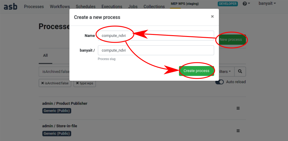
Go to Processes -> New Process and create a new process similar to:
This will bring you to the process's page. Click twice (asks for a confirmation) on New version, then drag and drop both process wrapper and requirements files:
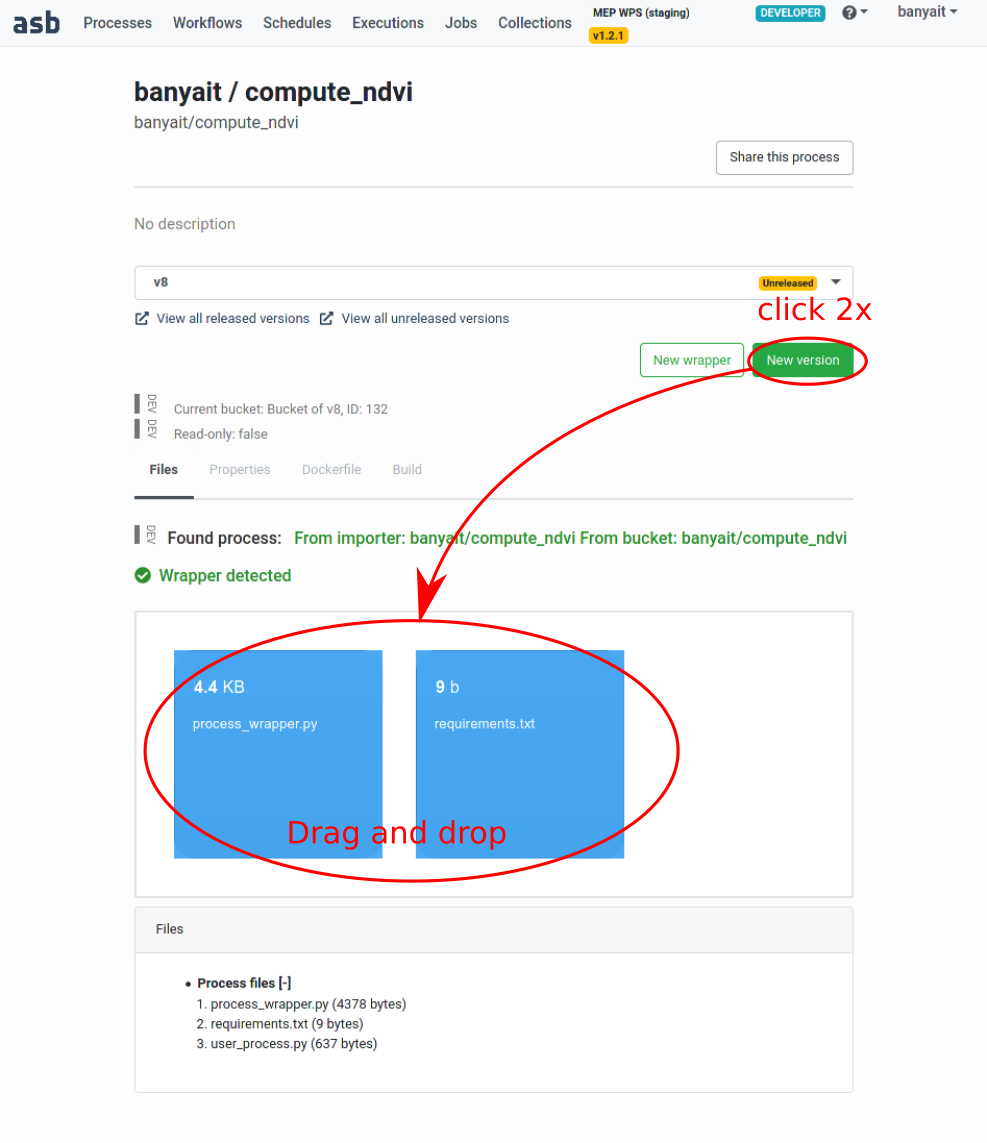
Figure: uploading the wrapper and requirements
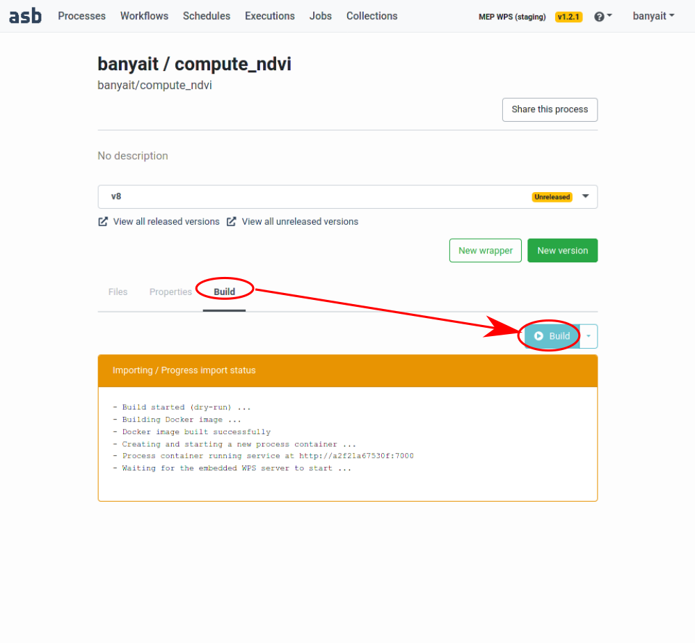
Next the process needs to be built (assembling the docker container), this is done by clicking on the build tab and Build:
When the progress becomes green, the process is ready to be released via Build and release. When that is finished (progress becomes green again), the process is ready to be used in workflows.
Once again, this is a builtin pocess. It waits until all the upstream dynamic processes finish and puts 'success' on its single output if there were no failures.
This process will lookup the outputs of the compute_ndvis on the file system, and combine them by always choosing the maximum value at the same pixels. The procedure of creating this process is very similar to the one of compute_ndvi:
- create an empty process wrapper with:
- Inputs: status and outputFile, both user strings. Status will receive the information from the joiner if all went well so far and outputFile will store the filename of the merged result.
- Outputs: result user string (outputFile repeated)
- same resources as compute_ndvi
- we will also need the same requirements.txt file
The complete code process wrapper for the collector looks like this:
#!/usr/bin/python

import logging
import xarray
from pathlib import Path
import glob

# --------------------------------------------------------------------------------------
# Save this code in file "process_wrapper.py" and adapt as indicated in inline comments.
#
# Notes:
#  - This is a Python 3 script.
#  - The inputs will be given values by name, thus their order has no importance ...
#  - ... except that the inputs with a default value must be listed last.
#  - Parameter names are automatically converted into valid Python variable names.
#  - Any empty line or line starting with a '#' character will be ignored.
# --------------------------------------------------------------------------------------

logger = logging.getLogger(__name__)
logging.basicConfig(level=logging.INFO)

def execute(out_dir, status, outputFile):
    """
    Inputs:
    status -- status -- 45/User String
    outputFile -- outputFile -- 45/User String

    Outputs:
    result -- result -- 95/User String

    Main Dependency:
    mep-wps/uc-bundle-1

    Software Dependencies:
    pywps-4

    Processing Resources:
    ram -- 4
    disk -- 10
    cpu -- 1
    gpu -- 0
    """

    # ----------------------------------------------------------------------------------
    # Insert your own code below.
    # The files generated by your code must be stored in the "out_dir" folder.
    # Only the content of that folder is persisted in the datastore.
    # Give appropriate values to the output parameters. These will be passed to the next
    # process(es) following the workflow connections.
    # ----------------------------------------------------------------------------------

    logger.info("Starting...")

    if status=="success":

        # combine using max
        rxr=None
        searchPath=str(Path(str(out_dir).replace('/scratch/','/data/outputs/'),'..').resolve())+"_child/*/outputs/part_*"
        logger.info("Searching in: "+searchPath)
        for ifile in glob.glob(searchPath):
            with open(ifile,'r') as f:
                logger.info("Merging: "+ifile)
                ds=xarray.open_dataset(ifile, engine='h5netcdf')
                iarr=ds.to_array(dim='band')
                if rxr is None:
                    rxr=iarr
                    rxr=rxr.assign_coords({'band':['maxNDVI']})
                else:
                    rxr=xarray.concat([rxr,iarr], dim='band',join='outer').max(dim='band').expand_dims({'band':['maxNDVI']})

        # write to netcdf
        if rxr is not None:
            if rxr.dims[-2]=='x' and rxr.dims[-1]=='y':
                l=list(rxr.dims[:-2])
                rxr=rxr.transpose(*(l+['y','x']))
            result=rxr.to_dataset('band')
            result.to_netcdf(str(Path(out_dir,outputFile)), engine='h5netcdf')
            logger.info("Combined result saved to: "+str(Path(out_dir,outputFile)))
            outputFile=str(Path(str(out_dir).replace('/scratch/','/'),'outputs',outputFile))
        else:
            outputFile="<EMPTY>"
            logger.info("Combined result is empty, skipping")

    logger.info("Finished...")

    # ----------------------------------------------------------------------------------
    # The wrapper must return a dictionary that contains the output parameter values.
    # ----------------------------------------------------------------------------------
    return {
        "result": outputFile
    }
Where the first part is looking up the inputs on the file system. When a process finishes, it's out_dir contents are moved to a permanent storage. The line setting searchPath computes the permanent path from out_dir. Note the part_ prefix in the file name:
searchPath=str(Path(str(out_dir).replace('/scratch/','/data/outputs/'),'..').resolve())+"_child/*/outputs/part_*"
The next is the actual max merging. The glob function does the wildcard search over searchPath. Xarray provides an easy to use functionality to merge by coordinate values on partially overlapping domains (concat(...)). Collector uses that when appending the first chunk with the subsequent ones, while taking their maximum (by calling max(...) in band direction).
for ifile in glob.glob(searchPath):
    with open(ifile,'r') as f:
        ds=xarray.open_dataset(ifile, engine='h5netcdf')
        iarr=ds.to_array(dim='band')
        if rxr is None:
            rxr=iarr
            rxr=rxr.assign_coords({'band':['maxNDVI']})
        else:
            rxr=xarray.concat([rxr,iarr], dim='band',join='outer').max(dim='band').expand_dims({'band':['maxNDVI']})
The rest is really just saving the result to file or communicate if the result is empty:
if rxr is not None:
    if rxr.dims[-2]=='x' and rxr.dims[-1]=='y':
        l=list(rxr.dims[:-2])
        rxr=rxr.transpose(*(l+['y','x']))
    result=rxr.to_dataset('band')
    result.to_netcdf(str(Path(out_dir,outputFile)), engine='h5netcdf')
    outputFile=str(Path(str(out_dir).replace('/scratch/','/'),'outputs',outputFile))
else:
    outputFile="<EMPTY>"
Note: with a bit of modifications this process could easily be turned into a general 'temporal maximum' function, which could take other inputs rather than the Sentinel-2 ones generated by compute NDVI.
Again: similar how compute_ndvi was prepared: create and build a new process called collect_and_max.
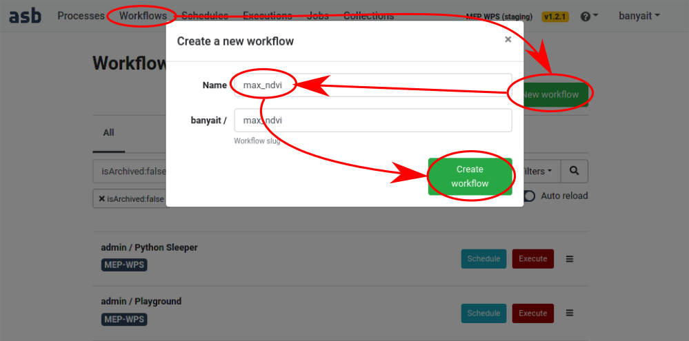
On the Workflows tab click New workflow, give it a name and Create workflow:
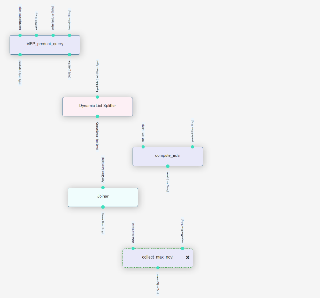
This will bring you to the workflow's page. On the left side, in the search bar type MEP, this will filter all processes and will show the ones having MEP in their name. Add the latest (v8 in this case) version by hovering over it and clicking on the '+' sign that appears.
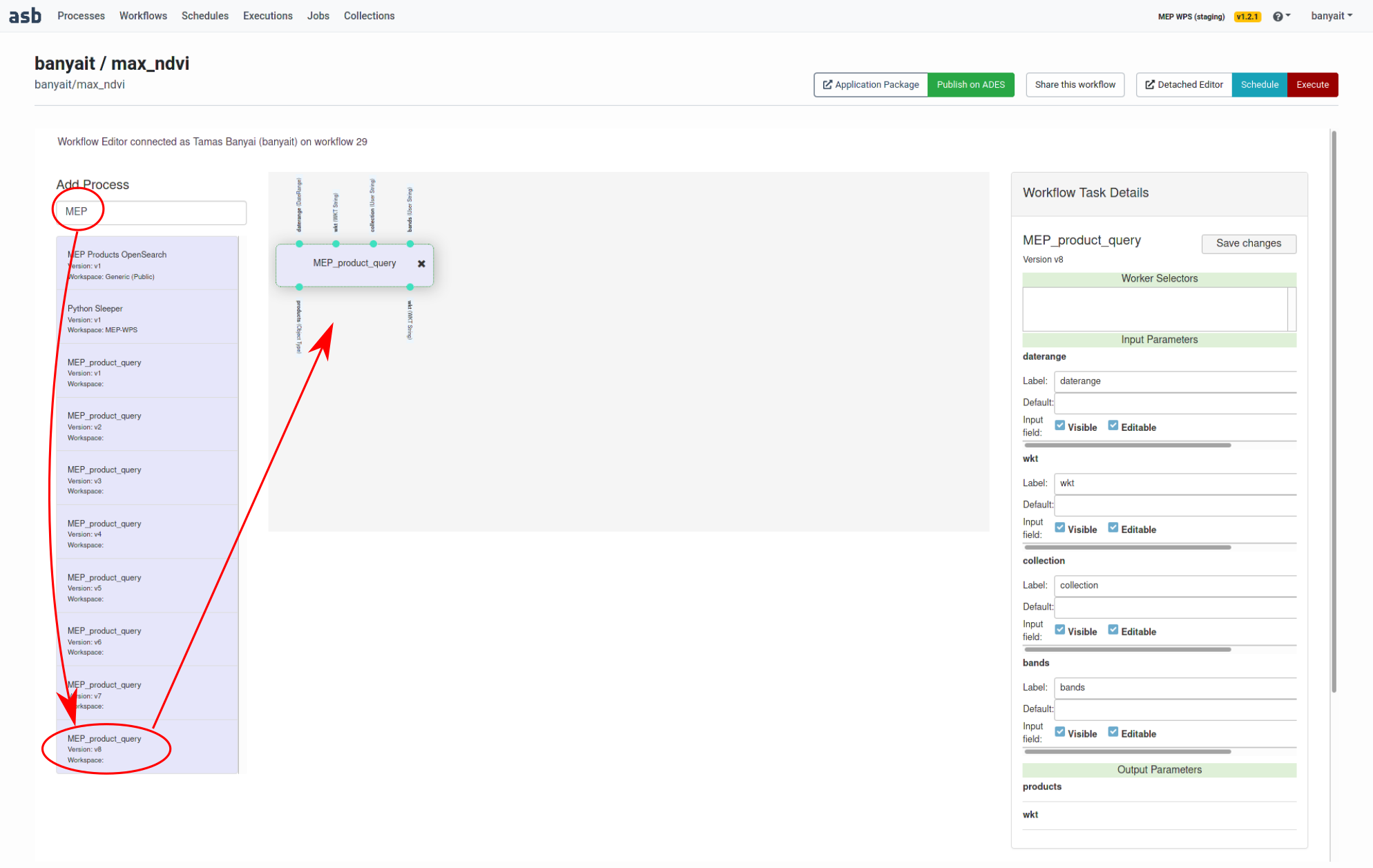
Figure: adding the first process to the workflow
Similarly, add (always the latest versions) these processes to the workflow:
- Dynamic List Splitter
- compute_ndvi
- Joiner
- collect_and_max
The canvas should look like this:
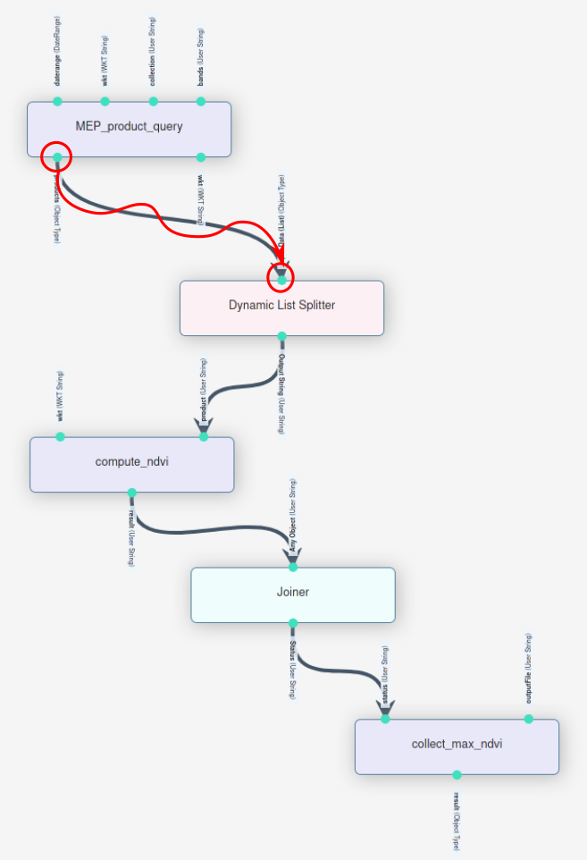
Next, connect the inputs to the outputs (by click and drag by the green dots) as shown:
The leftover free inputs have to be specified. This can be done either by filling out the missing fields when executing the workflow or specifying default values. Let's set default values to values that do not change often:
- collection: urn:eop:VITO:TERRASCOPE_S2_TOC_V2
- bands: ["B04","B08"]
- outputFile: mergedResults.nc
This is done by clicking on the process, filling out the values on the right side and clicking Save Changes:
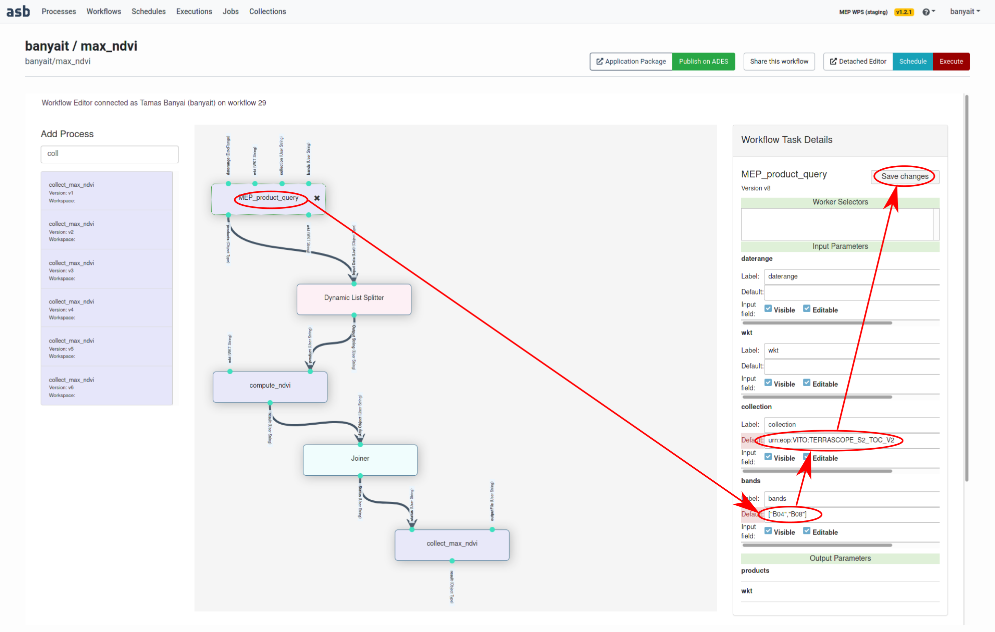
Figure: setting default values for a process
Similarly, set the outputFile field for the collect_and_max process.
This concludes setting up processes and workflows. What remains is to produce some results!
In workflows select the desired workflow (I named mine max_ndvi) and click on Execute in the top right corner. This will bring up the inputs page.
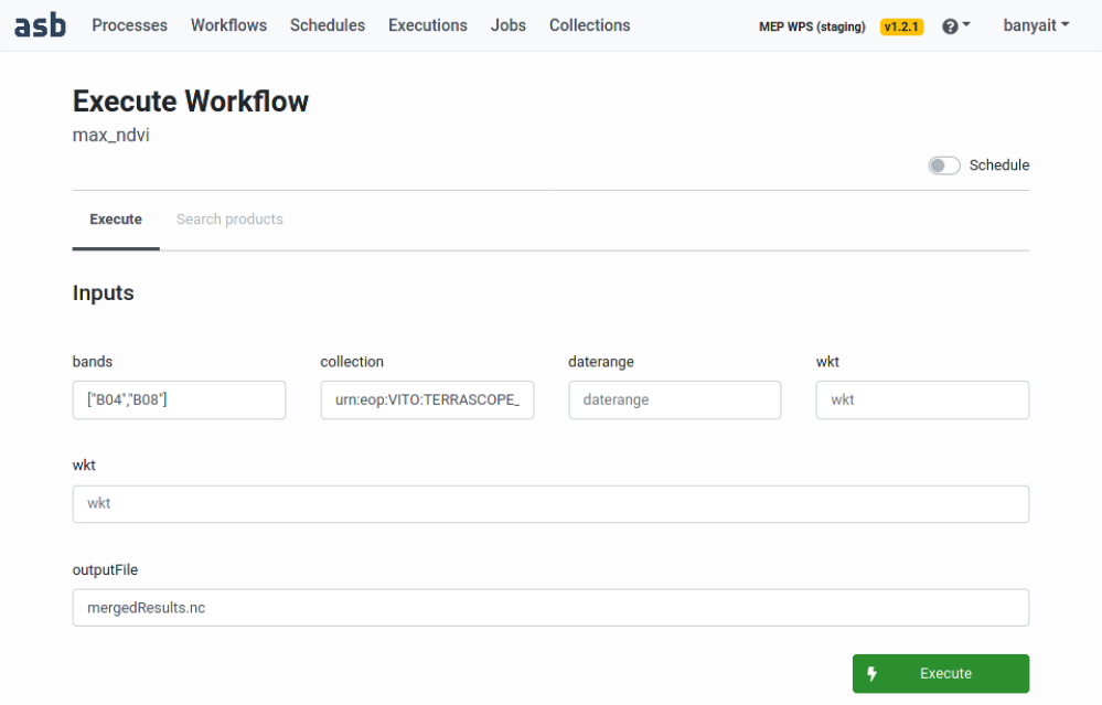
Figure: pre-filled default fields for an execution
The fields that have defaults already appear pre-filled. Those can be changed of course but let's just fill the empty fields. Note that wkt has to be filled twice: this is because a current limitation that the dynamically splitted processes can't be connected to the processes upstream of the splitter. Once all inputs are in order, click Execute to start the computation:
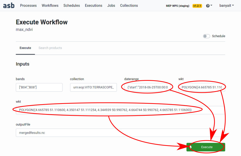
Figure: all fields completed for an execution
The progress is displayed in the Executions tab:
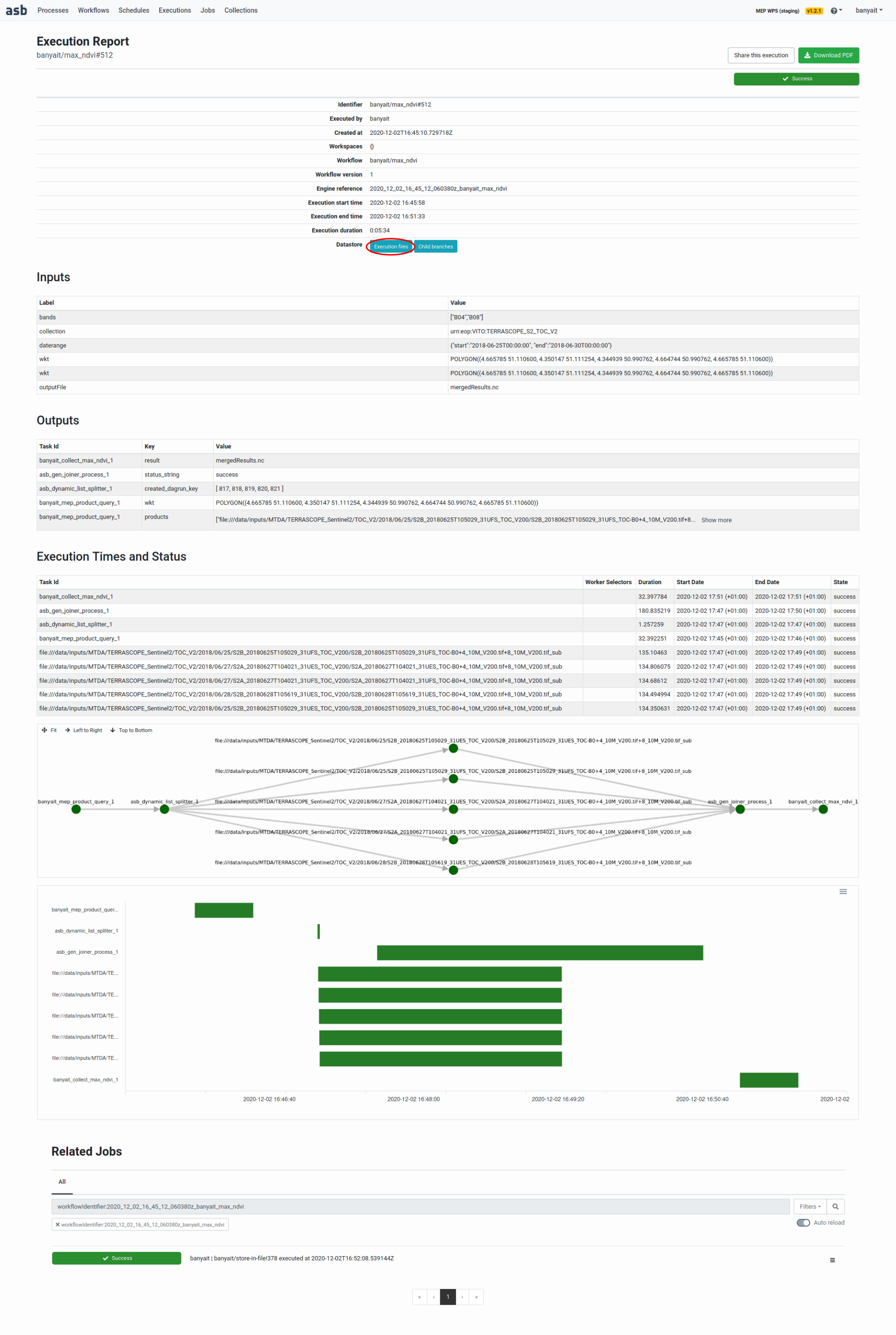
Once it is completed (either green if successful or red if failed), the execution report becomes available:

Figure: execution successfully finished
The execution summary will print out various details of the job, such as:
- All outputs of all processes
- Execution graph
- Timing of the processes
An important output is the result field of collect_and_max, which contains the path to the file with the merged results. Currently, there are two ways to access this file:
- by logging into the Terrascope user VM, which have to be requested separately at terrascope.be
- or by copying via SFTP
We will use the second option. Since this tutorial was written on linux, the simplest is to use the following command from a terminal:
sftp <USER>@probavmepftp.vgt.vito.be:/Private/<USER>/<RESULT_FIELD> <PATH_TO>/<DESTINATION>
Where:
- : user name
- <RESULT_FIELD>: the contents of the result field
- <PATH_TO>/: the path and filename on your computer where to save the file to.
Note: if you don't feel comfortable using terminal, there are many graphical SFTP clients (WinSCP,gFTP,...) available.
In this workflow the merged result is saved as NetCDF, which can for example be visualized with QGIS:
qgis <PATH_TO>/<DESTINATION>
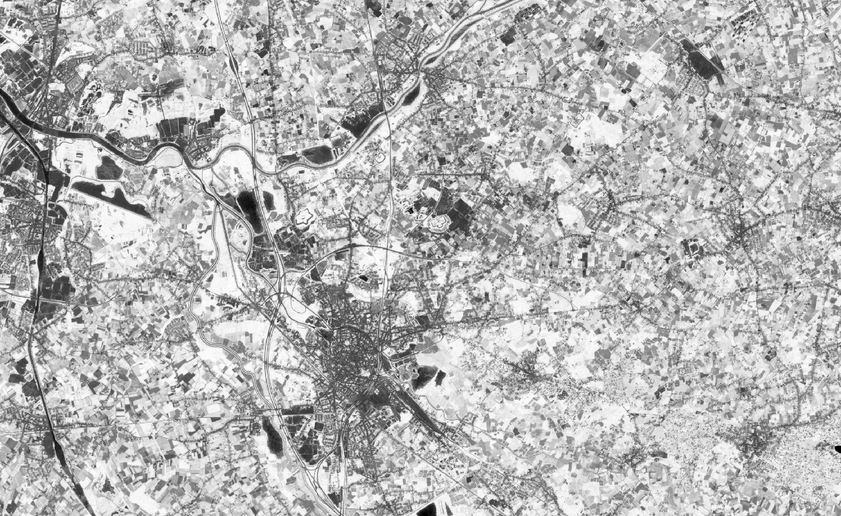
Figure: final result, maximum NDVI
That's it, well done!
In this concrete example the MEP query resulted in 5 B4/B8 pairs of images. Those are from the Sentinel-2 tiles 31UES and 31UFS at various days in the range and were processed independently in a parallel fashion, thanks to the dynamic splitter. Finally, the max collector produced this combined result from the parts.
- developed two processes for calculating NDVI and it's max combiner
- using the above two and also reusing some existing processes, built a worklfow for obtaining max NDVI
- successfully run the calculation using that workflow
- how to create processes
- how to create workflows
- how to execute workflows
