Leonard 7/3/2020
============================================
This document is submitted for Coursera Reproducible Research Project I.
This assignment makes use of data from a personal activity monitoring device. This device collects data at 5 minute intervals through out the day. The data consists of two months of data from an anonymous individual collected during the months of October and November, 2012 and include the number of steps taken in 5 minute intervals each day.
The data for this assignment can be downloaded from the course web site:
Activity Monitoring data [52K]
The variables included in this dataset are:
-
steps: Number of steps taking in a 5-minute interval (missing values are coded as NA)
-
date: The date on which the measurement was taken in YYYY-MM-DD format
-
interval: Identifier for the 5-minute interval in which measurement was taken
The dataset is stored in a comma-separated-value (CSV) file and there are a total of 17,568 observations in this dataset.
To download the data to your working directory, use download.file()
and name the destfile according to your desire. After that, unzip the
file using the unzip function
url <- "https://d396qusza40orc.cloudfront.net/repdata%2Fdata%2Factivity.zip"
if(!file.exists("activity.csv")){
download.file(url, destfile = "./dataproj1.zip")
unzip("./dataproj1.zip")}After the unzipped file is in your working directory, load it into R and
assign it into variable using the fread function from data.table
package. Don’t forget to assign “NA” as the na.strings argument.
library(data.table)
dataRaw <- fread("./activity.csv", na.strings = "NA")
Check the data information using simple function such as head, dim,
and str
Using dim to check the dimensions of the data.
dim(dataRaw)## [1] 17568 3
Using head to check the upper rows of the data.
```r
head(dataRaw)
## steps date interval
## 1: NA 2012-10-01 0
## 2: NA 2012-10-01 5
## 3: NA 2012-10-01 10
## 4: NA 2012-10-01 15
## 5: NA 2012-10-01 20
## 6: NA 2012-10-01 25
Using str to see the strucutre of the data.
str(dataRaw)## Classes 'data.table' and 'data.frame': 17568 obs. of 3 variables:
## $ steps : int NA NA NA NA NA NA NA NA NA NA ...
## $ date : chr "2012-10-01" "2012-10-01" "2012-10-01" "2012-10-01" ...
## $ interval: int 0 5 10 15 20 25 30 35 40 45 ...
## - attr(*, ".internal.selfref")=<externalptr>
Since the date column isn’t in date format, we shall change it into
date format using as.Date function.
dataRaw$date <- as.Date(dataRaw$date, format = "%Y-%m-%d")Before analyzing the data, we will remove the NA values and take only the complete data. Since analysis will be split into multiple part (With or Without Removing data), we shall create 2 data to fulfill this demand.
WONAdata <- dataRaw[complete.cases(dataRaw), ] ## this will be the data without NA, To make this plot, we’ll use base plotting system. First, calculate
steps based on date using aggregate function and assign it into
variable named agg.
agg1 <- aggregate(steps ~ date, data = WONAdata, FUN = sum)
head(agg1)
## date steps
## 1 2012-10-02 126
## 2 2012-10-03 11352
## 3 2012-10-04 12116
## 4 2012-10-05 13294
## 5 2012-10-06 15420
## 6 2012-10-07 11015
After that, simply call hist function and assign steps as the
argument.
hist(agg1$steps, main = "Histogram of The Total Number Of Steps Taken Each Day")Next we will be calculating mean and median of the total number of steps taken per day.
Simply call mean and `median on our aggregated data.
Calculating Mean
mean(agg1$steps)## [1] 10766.19
Calculating Median
median(agg1$steps)## [1] 10765
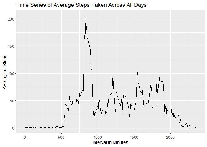
To plot a time series of average number of steps taken, we can use
aggregate function to calculate average steps taken across all days
based on interval variable.
agg3 <- aggregate(steps ~ interval, data = WONAdata, mean)Plot agg3 using ggplot and line as the plotting method.
library(ggplot2)
ggplot(agg3, aes(x=interval, y= steps)) + geom_line() + labs(title = "Time Series of Average Steps Taken Across All Days", x = "Interval in Minutes", y= "Average of Steps")
To answer which 5-minute interva has the maximum average value, simply
use the which.max function as follows.
paste ("The Answer is the ",
as.character(agg3$interval[which.max(agg3$steps)])
        ,"-minute interval" , sep ="")
## [1] "The Answer is the 835-minute interval"
Note that there are a number of days/intervals where there are missing
values NA. The presence of missing days may introduce bias into some
calculations or summaries of the data.
First, we shall check the number of missing values in each column using these following lines.
summary(dataRaw)## steps date interval
## Min. : 0.00 Min. :2012-10-01 Min. : 0.0
## 1st Qu.: 0.00 1st Qu.:2012-10-16 1st Qu.: 588.8
## Median : 0.00 Median :2012-10-31 Median :1177.5
## Mean : 37.38 Mean :2012-10-31 Mean :1177.5
## 3rd Qu.: 12.00 3rd Qu.:2012-11-15 3rd Qu.:1766.2
## Max. :806.00 Max. :2012-11-30 Max. :2355.0
## NA's :2304
To deal with missing values, we simply assign average values of steps taken on that day to fill the missing steps value.
Since we’ll be comparing with and without NA’s data, recall that
dataRaw variable is the variable with NA values in it, To avoid
confusion, let’s create a new variable imputeData , this will be our
data with NA values filled.
imputeData <- dataRaw
for (i in 1:nrow(imputeData)) {
    if(is.na(imputeData$steps[i])){
        imputeData$steps[i] <- agg3$steps[agg3$interval == imputeData$interval[i]]
    }
}
Let’s view some of the steps column on this data.
print(imputeData)## steps date interval
## 1: 1.7169811 2012-10-01 0
## 2: 0.3396226 2012-10-01 5
## 3: 0.1320755 2012-10-01 10
## 4: 0.1509434 2012-10-01 15
## 5: 0.0754717 2012-10-01 20
## ---
## 17564: 4.6981132 2012-11-30 2335
## 17565: 3.3018868 2012-11-30 2340
## 17566: 0.6415094 2012-11-30 2345
## 17567: 0.2264151 2012-11-30 2350
## 17568: 1.0754717 2012-11-30 2355
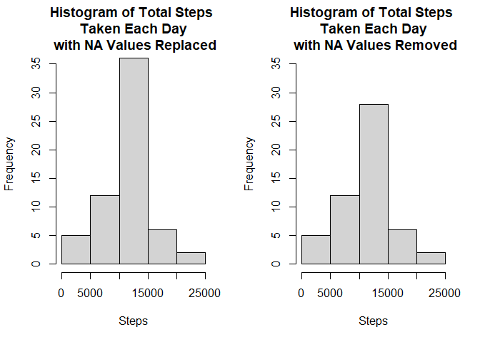
Lets make a histogram of steps taken each day using this newly data.
par(mfrow = c(1,2))
agg4 <- aggregate(steps ~ date, data = imputeData, sum)

hist(agg4$steps, main = "Histogram of Total Steps \n Taken Each Day \n with NA Values Replaced", ylim=c(0,35),  xlab = "Steps")

hist(agg1$steps, main = "Histogram of Total Steps \n Taken Each Day \n with NA Values Removed",  ylim=c(0,35), xlab = "Steps")
For the mean and median, we’ll again use the aggregate function to calculate the values.
agg5 <- aggregate(steps ~ date, data = imputeData, FUN = sum)After having the calculated data for, we shall calculate both mean and median.
Calculating Mean
mean(agg1$steps)## [1] 10766.19
Calculating Median
median(agg1$steps)## [1] 10765
As you can see from the results, imputing NA values didn’t affect the median and mean value significantly.
For this part the weekdays() function may be of some help here. Use
the dataset with the filled-in missing values for this part.
First, change the date column data into date format.
imputeData$date <- as.Date(imputeData$date) Second determine whether date is weekdays or weekend.
library(lubridate)##
## Attaching package: 'lubridate'
## The following objects are masked from 'package:data.table':
##
## hour, isoweek, mday, minute, month, quarter, second, wday, week,
## yday, year
## The following objects are masked from 'package:base':
##
## date, intersect, setdiff, union
imputeData$day <- weekdays(imputeData$date)
for(i in 1:nrow(imputeData)){
        if(imputeData[i, ]$day %in% c("Saturday", "Sunday")){
                imputeData[i, ]$day <- "Weekend"
        }
        else {
         imputeData[i, ]$day <- "Weekday"
        }
}
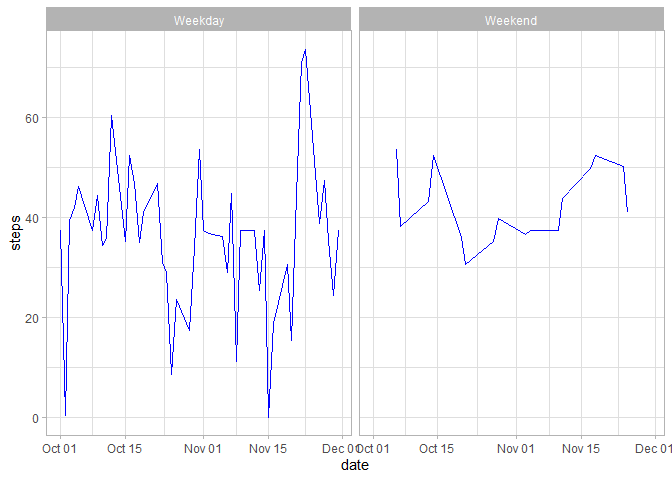
Lastly, we shall create another variable to store average steps taken
based on two parameters, date and day.
agg6 <- aggregate(steps ~ date + day, imputeData, mean)After that, plot the data using ggplot plotting system as follows.
ggplot(agg6, aes(x = date, y =steps)) + facet_wrap(.~day) + geom_line(color = "blue") + theme_light()


