Community Detection

A library for Community Detection in graphs.

Introduction

Community Detection (or Community Search) is the process of finding sets of densely connected nodes in a graph which are structurally close to each other. We use the following algorithms in this library:

Spectral Clustering
Louvain Method
Girvan-Newman algorithm

Application

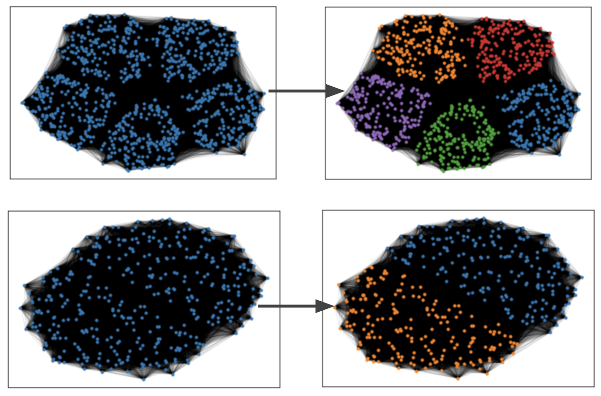
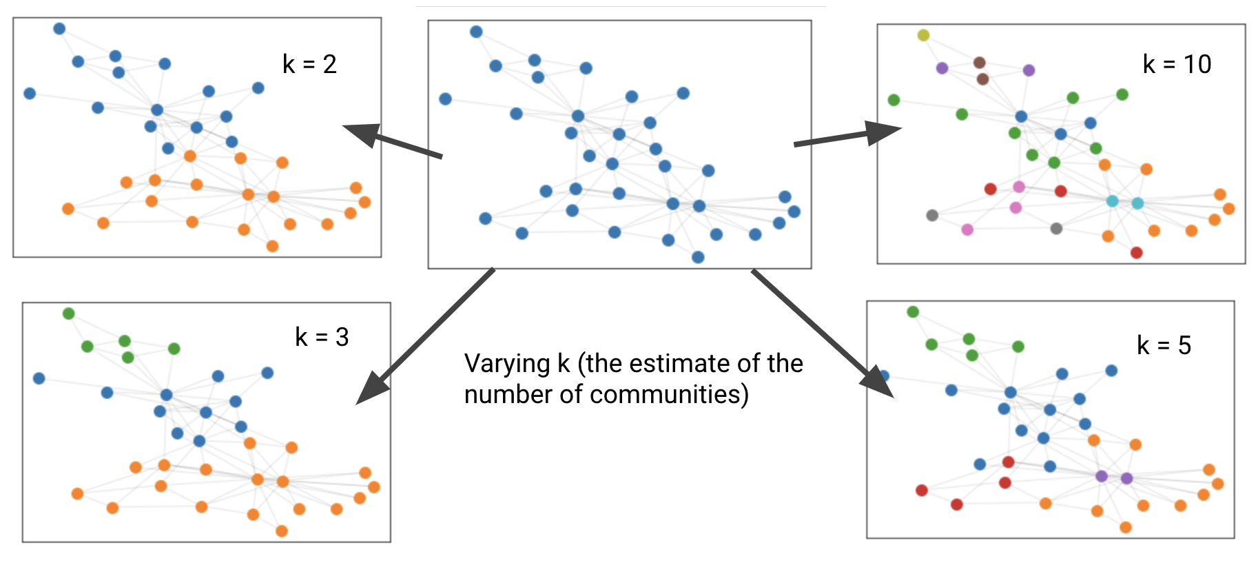
We tested our library on the Planted L-Partition Model (specifications in code) and Zachary’s Karate Club Network to visualize the results.

Planted L-Partition Model

Zachary’s Karate Club Network

Algorithms and Usage

Spectral Clustering

Test on Planted L Partition Model

import networkx as nx
from cdet.spectral_clustering import visualize_graph, spectral_clustering

# Color scheme
COLORS = \
    ["tab:blue", "tab:orange", "tab:green", 
     "tab:red", "tab:purple", "tab:brown", 
     "tab:pink", "tab:gray", "tab:olive", 
     "tab:cyan"]

# Create Planted L-Partition graph 
K = 5
NODES_PER_BUCKET = 200
P_IN = 0.8
P_OUT = 0.1

G_pl = nx.generators.community.planted_partition_graph(K, 
						       NODES_PER_BUCKET, 
						       P_IN, 
						       P_OUT)
pos_pl = nx.spring_layout(G_pl)

# Visualize base graph
visualize_graph(G_pl, pos_pl, edge_alpha=0.1, node_size=10, labels=False)

# Use Spectral Clustering and visualize
labels_dict = spectral_clustering(G_pl, 
                                  K, 
                                  pos_pl, 
                                  COLORS, 
                                  laplacian_type="symmetric", 
                                  edge_alpha=0.1, 
                                  node_size=10, 
                                  labels=False)

Test on Zachary’s Karate Club Network

# Generate Zachary's Karate Club graph
G_kk = nx.karate_club_graph()
pos_kk = nx.spring_layout(G_kk)

# Visualize base graph
visualize_graph(G_kk, pos_kk)

# Use Spectral clustering and visualize
labels_dict = spectral_clustering(G_kk, 
				  3, 
				  pos_kk, 
				  COLORS, 
				  laplacian_type="symmetric")

Louvain Method

Test on Planted L-Partition Model

import networkx as nx
from cdet.louvains import visualize_graph, louvains_method, plantedl

# Color scheme
COLORS = \
    ["tab:blue", "tab:orange", "tab:green", 
     "tab:red", "tab:purple", "tab:brown", 
     "tab:pink", "tab:gray", "tab:olive", 
     "tab:cyan"]

result = plantedl()

G = result[0]
pos = nx.spring_layout(G)

final_partition = result[1][0]
final_modularity = result[1][1]

labels_dict = {i: final_partition[i] for i in range(len(final_partition))}

# Visualize clustered graph
visualize_graph(G, pos, labels_dict=labels_dict, colors=COLORS, node_size=10)

Girvan-Newman

You can use the original Networkx visualization options to visualize the outcomes from the algorithms as well.

Test on Planted L-Partition Model

# Original Planted L-Partition Graph
G = nx.planted_partition_graph(5, 30, 0.8, 0.1)
pos = nx.spring_layout(G, k=0.1, iterations=30, scale=1.3)

# Visualize using networkx API
nx.draw_networkx_nodes(G, pos=pos)
nx.draw_networkx_labels(G, pos=pos)
nx.draw_networkx_edges(G, pos=pos, width=2, alpha=1, edge_color='k')
plt.show() 

# Planted L-Partition Graph graph with 2 communities
visualize_community_structure(num_communities=2, G)

VedangW/community-detection

Community Detection

Introduction

Application

Algorithms and Usage