ElementEmbeddings

The Element Embeddings package provides high-level tools for analysing elemental and ionic species embeddings data. This primarily involves visualising the correlation between embedding schemes using different statistical measures.

Documentation: https://wmd-group.github.io/ElementEmbeddings/
Examples: https://github.com/WMD-group/ElementEmbeddings/tree/main/examples

Motivation

Machine learning approaches for materials informatics have become increasingly widespread. Some of these involve the use of deep learning techniques where the representation of the elements is learned rather than specified by the user of the model. While an important goal of machine learning training is to minimise the chosen error function to make more accurate predictions, it is also important for us material scientists to be able to interpret these models. As such, we aim to evaluate and compare different atomic embedding schemes in a consistent framework.

Getting started

ElementEmbeddings's main feature, the Embedding class is accessible by importing the class.

Installation

The latest stable release can be installed via pip using:

pip install ElementEmbeddings

Alternatively, ElementEmbeddings is available via conda through the conda-forge channel on Anaconda Cloud:

conda install -c conda-forge elementembeddings

For installing the development or documentation dependencies via pip:

pip install "ElementEmbeddings[dev]"
pip install "ElementEmbeddings[docs]"

For development, you can clone the repository and install the package in editable mode. To clone the repository and make a local installation, run the following commands:

git clone https://github.com/WMD-group/ElementEmbeddings.git
cd ElementEmbeddings
pip install  -e ".[docs,dev]"

With -e pip will create links to the source folder so that changes to the code will be immediately reflected on the PATH.

Usage

For simple usage, you can instantiate an Embedding object using one of the embeddings in the data directory. For this example, let's use the magpie elemental representation.

# Import the class
>>> from elementembeddings.core import Embedding

# Load the magpie data
>>> magpie = Embedding.load_data('magpie')

We can access some of the properties of the Embedding class. For example, we can find the dimensions of the elemental representation and the list of elements for which an embedding exists.

# Print out some of the properties of the ElementEmbeddings class
>>> print(f'The magpie representation has embeddings of dimension {magpie.dim}')
>>> print(f'The magpie representation contains these elements: \n {magpie.element_list}') # prints out all the elements considered for this representation
>>> print(f'The magpie representation contains these features: \n {magpie.feature_labels}') # Prints out the feature labels of the chosen representation

The magpie representation has embeddings of dimension 22
The magpie representation contains these elements:
['H', 'He', 'Li', 'Be', 'B', 'C', 'N', 'O', 'F', 'Ne', 'Na', 'Mg', 'Al', 'Si', 'P', 'S', 'Cl', 'Ar', 'K', 'Ca', 'Sc', 'Ti', 'V', 'Cr', 'Mn', 'Fe', 'Co', 'Ni', 'Cu', 'Zn', 'Ga', 'Ge', 'As', 'Se', 'Br', 'Kr', 'Rb', 'Sr', 'Y', 'Zr', 'Nb', 'Mo', 'Tc', 'Ru', 'Rh', 'Pd', 'Ag', 'Cd', 'In', 'Sn', 'Sb', 'Te', 'I', 'Xe', 'Cs', 'Ba', 'La', 'Ce', 'Pr', 'Nd', 'Pm', 'Sm', 'Eu', 'Gd', 'Tb', 'Dy', 'Ho', 'Er', 'Tm', 'Yb', 'Lu', 'Hf', 'Ta', 'W', 'Re', 'Os', 'Ir', 'Pt', 'Au', 'Hg', 'Tl', 'Pb', 'Bi', 'Po', 'At', 'Rn', 'Fr', 'Ra', 'Ac', 'Th', 'Pa', 'U', 'Np', 'Pu', 'Am', 'Cm', 'Bk']
The magpie representation contains these features:
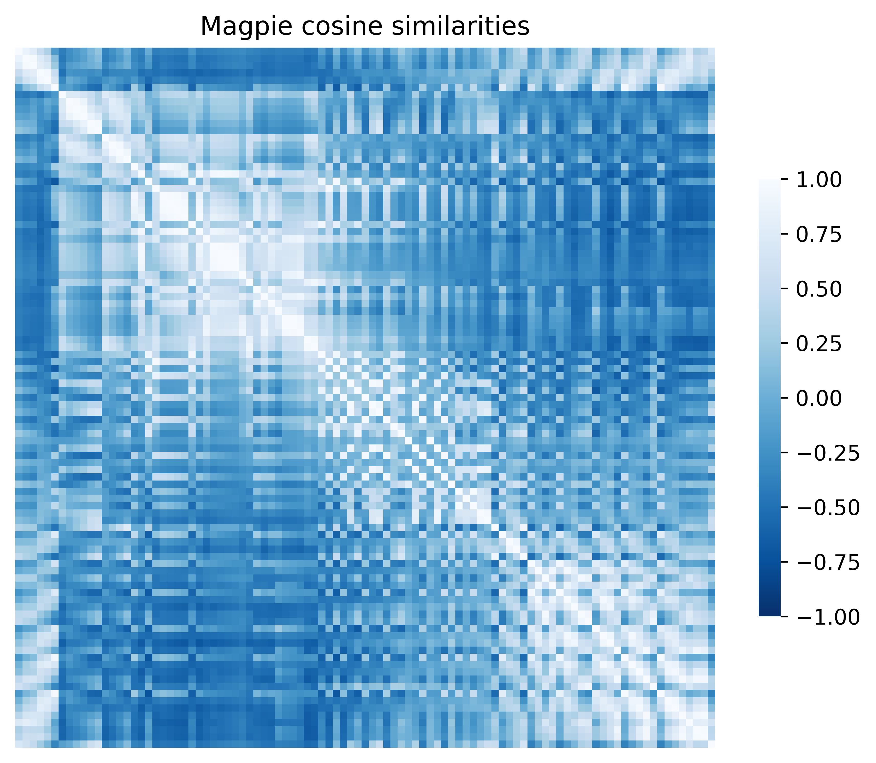
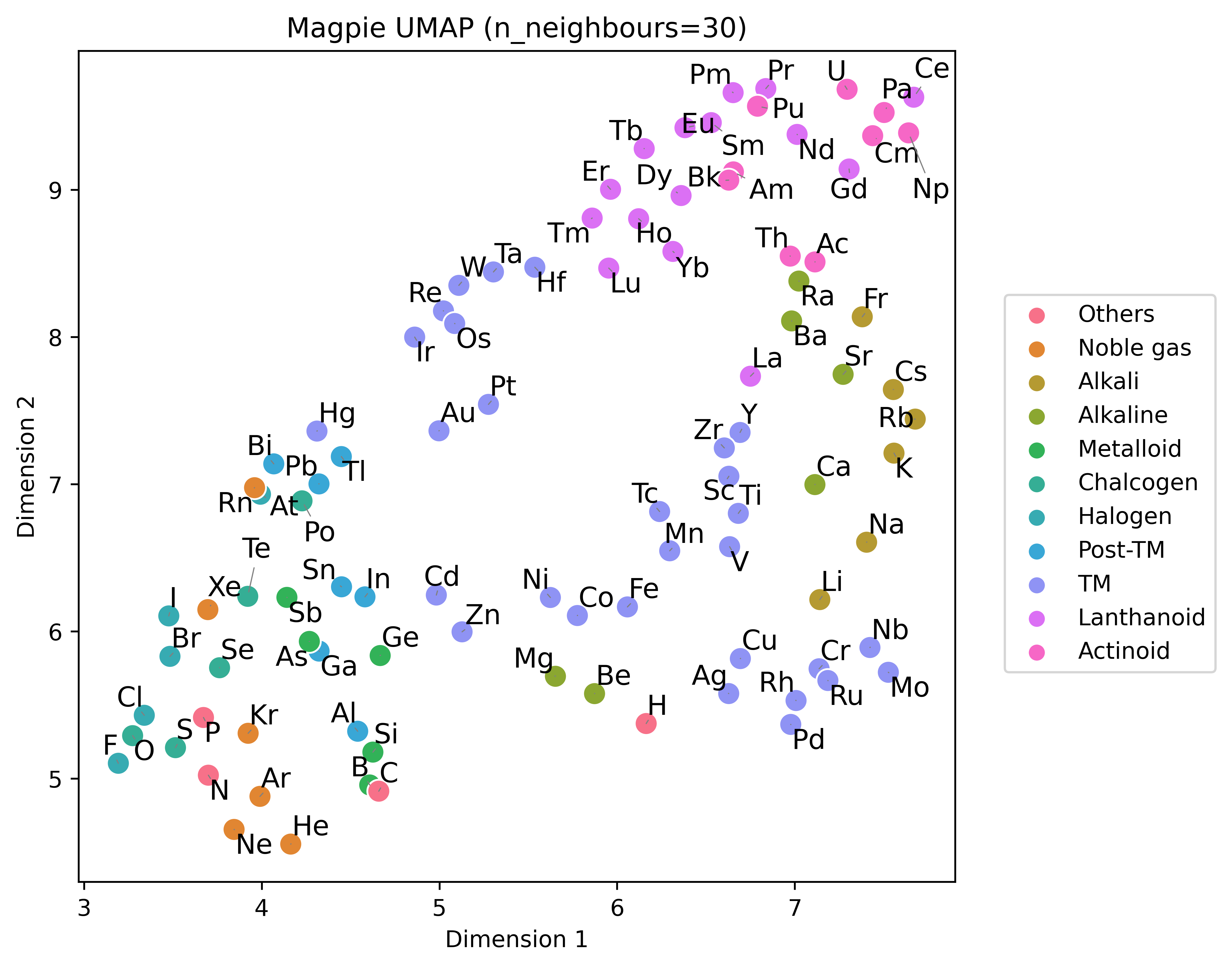
['Number', 'MendeleevNumber', 'AtomicWeight', 'MeltingT', 'Column', 'Row', 'CovalentRadius', 'Electronegativity', 'NsValence', 'NpValence', 'NdValence', 'NfValence', 'NValence', 'NsUnfilled', 'NpUnfilled', 'NdUnfilled', 'NfUnfilled', 'NUnfilled', 'GSvolume_pa', 'GSbandgap', 'GSmagmom', 'SpaceGroupNumber']

Plotting

We can quickly generate heatmaps of distance/similarity measures between the element vectors using heatmap_plotter and plot the representations in two dimensions using the dimension_plotter from the plotter module. Before we do that, we will standardise the embedding using the standardise method available to the Embedding class

from elementembeddings.plotter import heatmap_plotter, dimension_plotter
import matplotlib.pyplot as plt

magpie.standardise(inplace=True) # Standardises the representation

fig, ax = plt.subplots(1, 1, figsize=(6,6))
heatmap_params = {"vmin": -1, "vmax": 1}
heatmap_plotter(embedding=magpie, metric="cosine_similarity",show_axislabels=False,cmap="Blues_r",ax=ax, **heatmap_params)
ax.set_title("Magpie cosine similarities")
fig.tight_layout()
fig.show()

fig, ax = plt.subplots(1, 1, figsize=(6,6))

reducer_params={"n_neighbors": 30, "random_state":42}
scatter_params = {"s":100}

dimension_plotter(embedding=magpie, reducer="umap",n_components=2,ax=ax,adjusttext=True,reducer_params=reducer_params, scatter_params=scatter_params)
ax.set_title("Magpie UMAP (n_neighbours=30)")
ax.legend().remove()
handles, labels = ax1.get_legend_handles_labels()
fig.legend(handles, labels, bbox_to_anchor=(1.25, 0.5), loc="center right", ncol=1)

fig.tight_layout()
fig.show()

Compositions

The package can also be used to featurise compositions. Your data could be a list of formula strings or a pandas dataframe of the following format:

formula
CsPbI3
Fe2O3
NaCl
ZnS

The composition_featuriser function can be used to featurise the data. The compositions can be featurised using different representation schemes and different types of pooling through the embedding and stats arguments respectively.

from elementembeddings.composition import composition_featuriser

df_featurised = composition_featuriser(df, embedding="magpie", stats=["mean","sum"])

df_featurised

formula	mean_Number	mean_MendeleevNumber	mean_AtomicWeight	mean_MeltingT	mean_Column	mean_Row	mean_CovalentRadius	mean_Electronegativity	mean_NsValence	mean_NpValence	mean_NdValence	mean_NfValence	mean_NValence	mean_NsUnfilled	mean_NpUnfilled	mean_NdUnfilled	mean_NUnfilled	mean_GSvolume_pa	mean_GSbandgap	mean_GSmagmom	mean_SpaceGroupNumber	sum_Number	sum_MendeleevNumber	sum_AtomicWeight	sum_MeltingT	sum_Column	sum_Row	sum_CovalentRadius	sum_Electronegativity	sum_NsValence	sum_NpValence	sum_NdValence	sum_NfValence	sum_NValence	sum_NsUnfilled	sum_NpUnfilled	sum_NdUnfilled	sum_NUnfilled	sum_GSvolume_pa	sum_GSbandgap	sum_GSmagmom	sum_SpaceGroupNumber
CsPbI3	59.2	74.8	144.16377238	412.55	13.2	5.4	161.39999999999998	2.22	1.8	3.4	8.0	2.8000000000000003	16.0	0.2	1.4	0.0	1.6	54.584	0.6372	0.0	129.20000000000002	296.0	374.0	720.8188619	2062.75	66.0	27.0	807.0	11.100000000000001	9.0	17.0	40.0	14.0	80.0	1.0	7.0	0.0	8.0	272.92	3.186	0.0	646.0
Fe2O3	15.2	74.19999999999999	31.937640000000002	757.2800000000001	12.8	2.8	92.4	2.7960000000000003	2.0	2.4	2.4000000000000004	0.0	6.8	0.0	1.2	1.6	2.8	9.755	0.0	0.8442651200000001	98.80000000000001	76.0	371.0	159.6882	3786.4	64.0	14.0	462.0	13.98	10.0	12.0	12.0	0.0	34.0	0.0	6.0	8.0	14.0	48.775000000000006	0.0	4.2213256	494.0
NaCl	14.0	48.0	29.221384640000004	271.235	9.0	3.0	134.0	2.045	1.5	2.5	0.0	0.0	4.0	0.5	0.5	0.0	1.0	26.87041666665	1.2465	0.0	146.5	28.0	96.0	58.44276928000001	542.47	18.0	6.0	268.0	4.09	3.0	5.0	0.0	0.0	8.0	1.0	1.0	0.0	2.0	53.7408333333	2.493	0.0	293.0
ZnS	23.0	78.5	48.7225	540.52	14.0	3.5	113.5	2.115	2.0	2.0	5.0	0.0	9.0	0.0	1.0	0.0	1.0	19.8734375	1.101	0.0	132.0	46.0	157.0	97.445	1081.04	28.0	7.0	227.0	4.23	4.0	4.0	10.0	0.0	18.0	0.0	2.0	0.0	2.0	39.746875	2.202	0.0	264.0

The returned dataframe contains the mean-pooled and sum-pooled features of the magpie representation for the four formulas.

Development notes

Bugs, features and questions

Please use the issue tracker to report bugs and any feature requests. Hopefully, most questions should be solvable through the docs. For any other queries related to the project, please contact Anthony Onwuli by e-mail: anthony.onwuli16@imperial.ac.uk.

Code contributions

We welcome new contributions to this project. See the contributing guide for detailed instructions on how to contribute to our project.

Add an embedding scheme

The steps required to add a new representation scheme are:

Add data file to data/element_representations.
Edit docstring table in core.py.
Edit utils/config.py to include the representation in DEFAULT_ELEMENT_EMBEDDINGS and CITATIONS.
Update the documentation reference.md and README.md.

Developer

Anthony Onwuli (Department of Materials, Imperial College London)

References

A. Onwuli et al, "Ionic species representations for materials informatics"

H. Park et al, "Mapping inorganic crystal chemical space" Faraday Discuss. (2024)

A. Onwuli et al, "Element similarity in high-dimensional materials representations" Digital Discovery 2, 1558 (2023)