hyRelease generates release hydrofabric artifacts for use in NextGen.
The types of data in each release is actively being discussed
here.
For now, we are generating releases for HUC01 units and CAMELS basins. These are stored in a Lynker Technologies AWS bucket. If you have credentials to these, data can be accessed in a number of ways.
A general approach (implemented in R, but general in nature) in the
following way for an example CAMELS basin draining to NWIS gage
01435000.
In order to connect to S3, you need to authenticate. One way easiest method is to set environment variables in a working session like this:
Sys.setenv("AWS_ACCESS_KEY_ID"     = "XXXXX",
           "AWS_SECRET_ACCESS_KEY" = "XXXXX",
           "AWS_DEFAULT_REGION"    = "us-east-2")
Or sourcing it from a private file:
source("private/aws.R")Or setting them to the root of your system.
However you authenticate, our resources are stored in us-east-2 but
your access key IDs and secrets are individual.
For NGEN applications a number of file formats are needed including CSV, JSON, geoJSON, and gpkg. The first three of these are files that can be read directly, while a gpkg has some intereesting database capabilites.
First, lets see what files are in our CAMEL “bucket”. AWS does not have an explict folder structure so files are defined by a bucket, and can be reduced by the file prefix. So, lets first find the files in the CAMELS/gage_0143500 “directory”.
library(aws.s3)
library(data.table)
library(dplyr)

rbindlist(get_bucket(bucket = "formulations-dev", prefix = "CAMELS/gage_01435000"))$Key
#>  [1] "CAMELS/gage_01435000/"
#>  [2] "CAMELS/gage_01435000/crosswalks/"
#>  [3] "CAMELS/gage_01435000/crosswalks/crosswalk-mapping.json"
#>  [4] "CAMELS/gage_01435000/graph/"
#>  [5] "CAMELS/gage_01435000/graph/catchment_edge_list.json"
#>  [6] "CAMELS/gage_01435000/graph/flowpath_edge_list.json"
#>  [7] "CAMELS/gage_01435000/graph/waterbody_edge_list.json"
#>  [8] "CAMELS/gage_01435000/parameters/"
#>  [9] "CAMELS/gage_01435000/parameters/camels.csv"
#> [10] "CAMELS/gage_01435000/parameters/nwm.csv"
#> [11] "CAMELS/gage_01435000/parameters/waterbody-params.json"
#> [12] "CAMELS/gage_01435000/spatial/"
#> [13] "CAMELS/gage_01435000/spatial/catchment_data.geojson"
#> [14] "CAMELS/gage_01435000/spatial/flowpath_data.geojson"
#> [15] "CAMELS/gage_01435000/spatial/hydrofabric.gpkg"
#> [16] "CAMELS/gage_01435000/spatial/nexus_data.geojson"
Onec we know what files are avaialble, we can read any of them by selecting the correct driver:
The pattern for reading files is identical regardless of format, the correct reader simply needs to be defined:
csv_data = s3read_using(fread, object = "s3://formulations-dev/CAMELS/gage_01435000/parameters/nwm.csv")
glimpse(csv_data)
#> Rows: 17
#> Columns: 13
#> $ ID                             <chr> "cat-1", "cat-10", "cat-11", "cat-12", …
#> $ gw_Coeff                       <dbl> 0.005, 0.005, 0.005, 0.005, 0.005, 0.00…
#> $ gw_Zmax                        <dbl> 34.75653, 241.20125, 241.20125, 154.072…
#> $ gw_Expon                       <int> 1, 6, 6, 3, 6, 1, 6, 6, 3, 6, 3, 3, 3, …
#> $ `sp_bexp_soil_layers_stag=1`   <int> 3, 4, 4, 3, 4, 3, 4, 4, 3, 4, 3, 3, 3, …
#> $ `sp_dksat_soil_layers_stag=1`  <dbl> 1.651e-06, 5.490e-06, 4.064e-06, 4.625e…
#> $ `sp_psisat_soil_layers_stag=1` <dbl> 0.7590000, 0.4473704, 0.4573333, 0.4573…
#> $ `sp_smcmax_soil_layers_stag=1` <dbl> 0.5700271, 0.4202248, 0.4217215, 0.4265…
#> $ `sp_smcwlt_soil_layers_stag=1` <dbl> 0.08400000, 0.07142511, 0.07182244, 0.0…
#> $ sp_slope                       <dbl> 0.06858038, 0.06552054, 0.07023233, 0.0…
#> $ wf_IVGTYP                      <int> 11, 15, 11, 15, 11, 11, 11, 11, 11, 11,…
#> $ wf_ISLTYP                      <int> 4, 6, 6, 6, 6, 4, 6, 6, 4, 4, 4, 4, 6, …
#> $ fd_LKSATFAC <dbl> 986.9935, 1511.3626, 1683.4473, 1090.86…library(jsonlite)
json_data = s3read_using(read_json, object = "s3://formulations-dev/CAMELS/gage_01435000/parameters/waterbody-params.json", simplifyVector = TRUE)
glimpse(json_data[[1]])
#> Rows: 1
#> Columns: 21
#> $ lengthMap <chr> "4147956.1"
#> $ toID <int> 100000018
#> $ Hydroseq <int> 1
#> $ member_COMID <list> "4147956"
#> $ LevelPathID <int> 1
#> $ length_km <dbl> 5.0756
#> $ areasqkm <dbl> 11.4347
#> $ gages <chr> "01435000"
#> $ Qi <int> 0
#> $ MusK <int> 3600
#> $ MusX <dbl> 0.2
#> $ n <dbl> 0.055
#> $ So <dbl> 0.006
#> $ ChSlp <dbl> 0.36
#> $ BtmWdth <dbl> 8.608
#> $ time <int> 0
#> $ Kchan <int> 0
#> $ nCC <dbl> 0.11
#> $ TopWdthCC <dbl> 43.041
#> $ TopWdth <dbl> 14.347
#> $ Length_m <dbl> 5075.585library(sf)
## READ from geoJSON
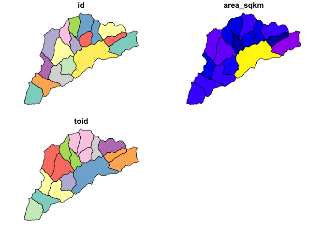
cat_data = s3read_using(read_sf, object = "s3://formulations-dev/CAMELS/gage_01435000/spatial/catchment_data.geojson")
plot(cat_data)## READ from GPKG
### find available layers
s3read_using(st_layers, object = "s3://formulations-dev/CAMELS/gage_01435000/spatial/hydrofabric.gpkg")
#> Driver: GPKG
#> Available layers:
#> layer_name geometry_type features fields
#> 1 catchments Polygon 17 3
#> 2 flowpaths Line String 17 7
#> 3 nexus Point 11 2
### call flowpaths layer
fp_data = s3read_using(st_read, object = "s3://formulations-dev/CAMELS/gage_01435000/spatial/hydrofabric.gpkg", "flowpaths")
#> Reading layer `flowpaths' from data source
#> `/private/var/folders/jc/ys3x7k814b9dnx208718f07m0000gn/T/RtmpSSuWOR/filea92274758c4c.gpkg'
#> using driver `GPKG'
#> Simple feature collection with 17 features and 7 fields
#> Geometry type: LINESTRING
#> Dimension: XY
#> Bounding box: xmin: 1746257 ymin: 2294474 xmax: 1763585 ymax: 2313553
#> Projected CRS: NAD83 / Conus Albers
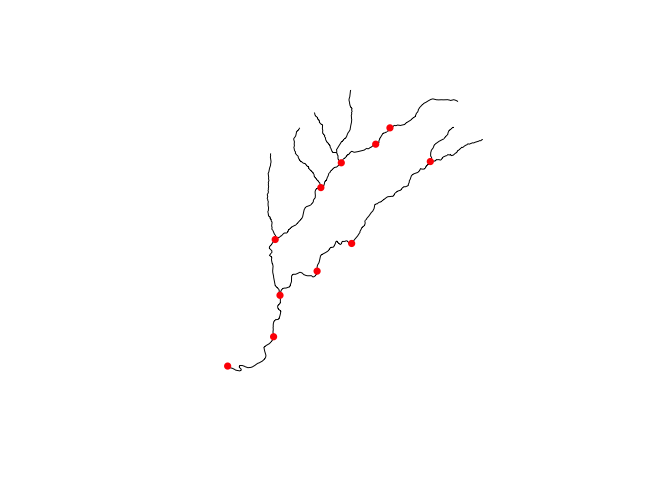
### plot and add nexus layer
{
plot(fp_data$geom)
plot(s3read_using(st_read, object = "s3://formulations-dev/CAMELS/gage_01435000/spatial/hydrofabric.gpkg", "nexus"), add = TRUE, pch = 16, col = "red")
}#> Reading layer `nexus' from data source
#> `/private/var/folders/jc/ys3x7k814b9dnx208718f07m0000gn/T/RtmpSSuWOR/filea922514e0d4f.gpkg'
#> using driver `GPKG'
#> Simple feature collection with 11 features and 2 fields
#> Geometry type: POINT
#> Dimension: XY
#> Bounding box: xmin: 1746257 ymin: 2294798 xmax: 1760023 ymax: 2310979
#> Projected CRS: NAD83 / Conus Albers
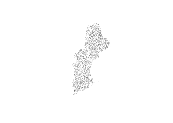
Because gpkgs are SQLite databases we can pass queries to the resource to extract exactly the features we need. For example, if we want to pull the just the junction nexus locations, we can do so.
junction_nex =  sf::st_read(
    dsn = "/vsis3/formulations-dev/hydrofabric/CONUS-hydrofabric/ngen-release/01a/2021-10-22/hydrofabric.gpkg",
    query = "SELECT * FROM nexus WHERE nexus_type == 'junction'")
#> Reading query `SELECT * FROM nexus WHERE nexus_type == 'junction'' from data source `/vsis3/formulations-dev/hydrofabric/CONUS-hydrofabric/ngen-release/01a/2021-10-22/hydrofabric.gpkg'
#>   using driver `GPKG'
#> Simple feature collection with 7401 features and 3 fields
#> Geometry type: POINT
#> Dimension:     XY
#> Bounding box:  xmin: 1827668 ymin: 2222999 xmax: 2242913 ymax: 3012187
#> Projected CRS: NAD83 / Conus Albers


plot(junction_nex$geom, pch = 16, cex = .1)
NOTE: The /vsis3/ path prefix allows us to access the gpkg as a
virtual dataset though GDALs
capabilites


