A Lightweight and Predictable Occupancy Representation for Short-range applications
Deformable Radar Polygon: A Lightweight and Predictable Occupancy Representation for Short-range Collision Avoidance,
Xiangyu Gao, Sihao Ding, Harshavardhan Reddy Dasari
IEEE Sensors Journal (arXiv 2203.01442)
@article{xiangyu2022deformable,
    title={Deformable Radar Polygon: A Lightweight and Predictable Occupancy Representation for Short-range Collision Avoidance},
    author={Xiangyu, Gao and Sihao, Ding and Reddy, Dasari Harshavardhan},
    journal={arXiv preprint arXiv:2203.01442},
    year={2022}}
(July 4, 2024) Code and sample data release.
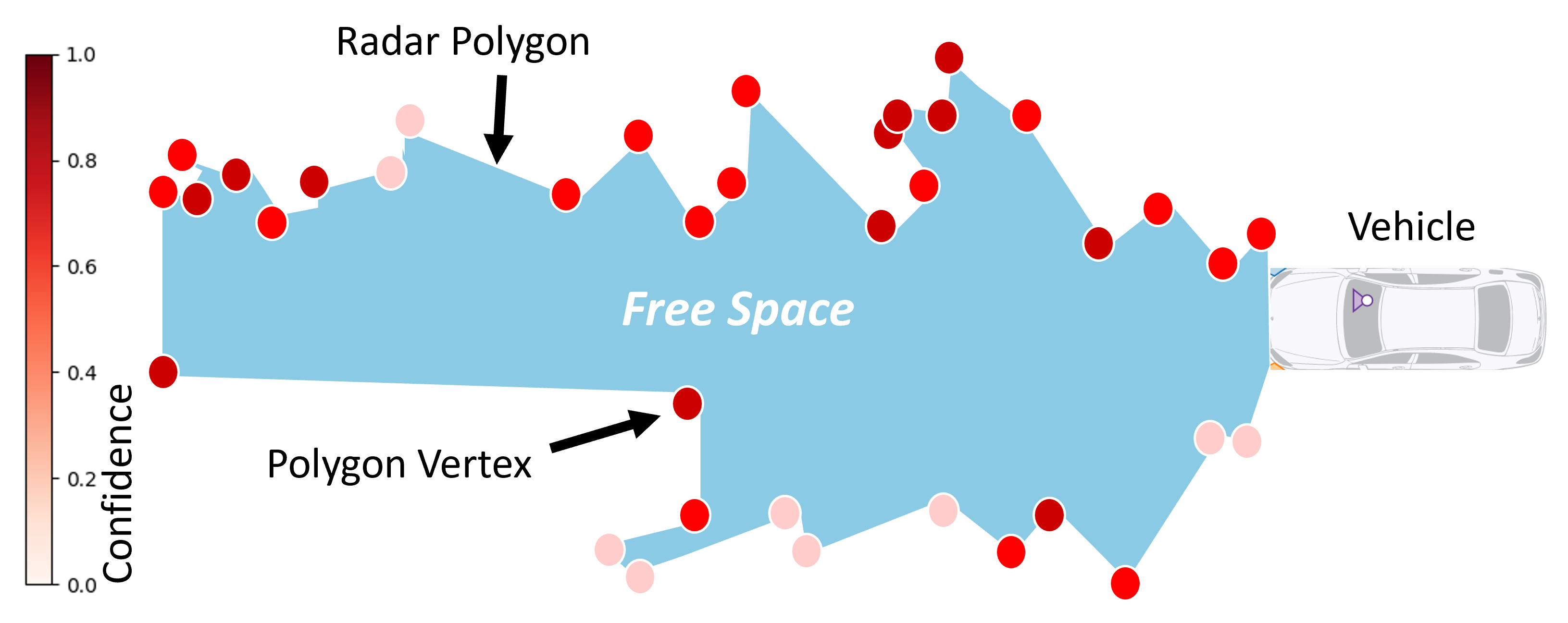
Inferring the drivable area in a scene is crucial for ensuring a vehicle avoids obstacles and facilitates safe autonomous driving. In this paper, we concentrate on detecting the instantaneous free space surrounding the ego vehicle, targeting shortrange automotive applications. We introduce a novel polygonbased occupancy representation, where the interior signifies free space, and the exterior represents undrivable areas for the egovehicle. The radar polygon consists of vertices selected from point cloud measurements provided by radars, with each vertex incorporating Doppler velocity information from automotive radars. This information indicates the movement of the vertex along the radial direction. This characteristic allows for the prediction of the shape of future radar polygons, leading to its designation as a “deformable radar polygon”. We propose two approaches to leverage noisy radar measurements for producing accurate and smooth radar polygons. The first approach is a basic radar polygon formation algorithm, which independently selects polygon vertices for each frame, using SNR-based evidence for vertex fitness verification. The second approach is the radar polygon update algorithm, which employs a probabilistic and tracking-based mechanism to update the radar polygon over time, further enhancing accuracy and smoothness. To accommodate the unique radar polygon format, we also designed a collision detection method for short-range applications. Through extensive experiments and analysis on both a self-collected dataset and the open-source RadarScenes dataset, we demonstrate that our radar polygon algorithms achieve significantly higher IoU-gt and IoUsmooth values compared to other occupancy detection baselines, highlighting their accuracy and smoothness.
All radar configurations and algorithm configurations are included in config.py.
Python 3.6, and libraries in requirements.txt.
-
From below Google Drive link download the sample data 'scene.pickle'.
https://drive.google.com/file/d/12NV46iAPfws4SVUuxyfHbsqE_BibqAyK/view?usp=sharingNote that the sample data is from the scene 143 of RadarScenes Dataset. You can try other data by downloading the RadarScenes, and read and save other scenes of data with the
read_radarscene_data.py. -
Relocate the pickle data under the project directory.
./deformable_radar_polygon_occupancy_representation/scene.pickle
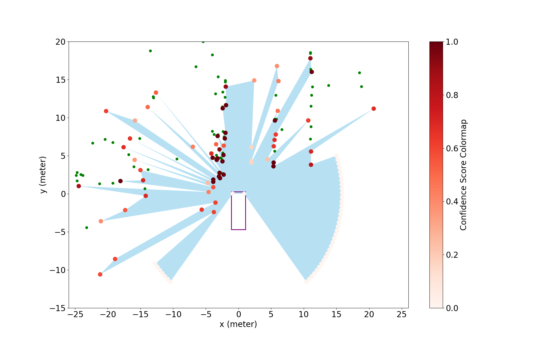
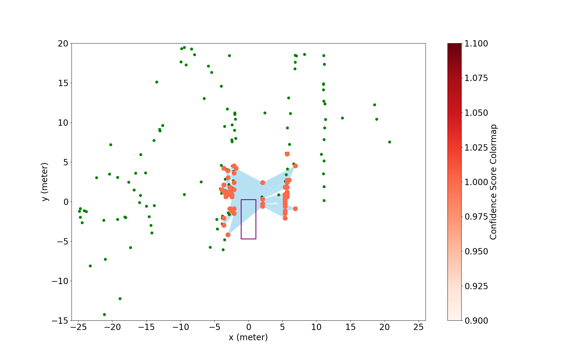
python polygon_radarscene_singleFrame.py
The polygon results are saved in ./res/results_polygon/radarScene143_poly as pickle file and their visualization is in ./res/results_bev/radarScene143_poly.
One example for 36-th frame is shown below:
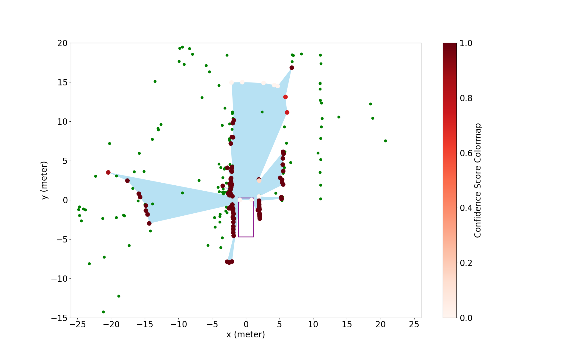
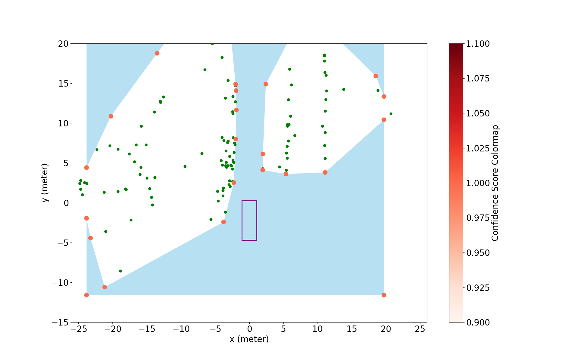
python polygon_radarscene_inverseSensor.py
The polygon results are saved in ./res/results_polygon/radarScene143_ism_poly as pickle file and their visualization is in ./res/results_bev/radarScene143_ism_poly.
One example for 36-th frame is shown below:
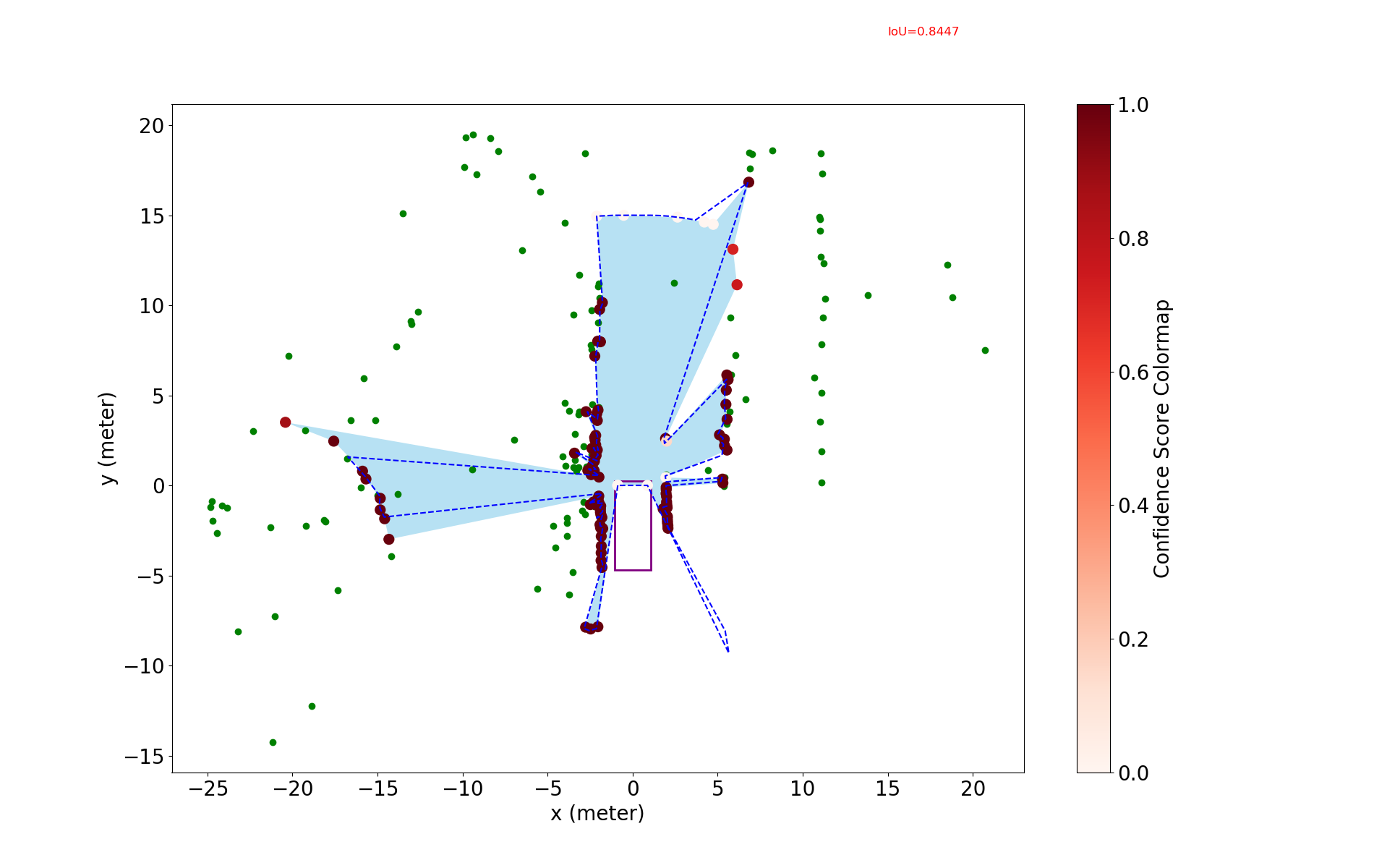
By enable is_withpred argument (i.e., set is_withpred=True) in polygon_radarscene_inverseSensor.py, then run it as below
python polygon_radarscene_inverseSensor.py
The polygon prediction results are visualization is in ./res/results_bev/radarScene143_ism_poly_pred using the dotted line.
One example for 36-th frame is shown below:
python meerpohl_polygon_radarscene.py
By default it is running with the algorithm in "Free-space Polygon Creation based on Occupancy Grid Maps for Trajectory Optimization Methods".
The polygon results are saved in './res/results_poly/radarScene143_meerpohl'* by default and their visualization is in ./res/results_bev/radarScene143_meerpohl by default.
One example for 36-th frame is shown below:
python ziegler_polygon_radarscene.py
By default it is running with the algorithm in "Trajectory planning for Bertha — A local, continuous method".
The polygon results are saved in ./res/results_poly/radarScene143_ziegler by default and their visualization is in ./res/results_bev/radarScene143_ziegler by default.
One example for 36-th frame is shown below:
python evaluate_radarScenes.py
You will get outputs as follows:
iou_gt for single-shot polygon is:  0.23665013401606833
iou_smooth for single-shot polygon is:  0.6891232717900692
conf_over_time for single-shot polygon is:  0.4402510760276303
iou_gt for ISM-based polygon is:  0.7444365353468597
iou_smooth for ISM-based polygon is:  0.8686911700136964
conf_over_time for single-shot polygon is:  0.8507623585611993
iou_gt for Meerpohl polygon is:  0.22913116594233784
iou_smooth for Meerpohl polygon is:  0.7055480795292997
conf_over_time for Meerpohl polygon is:  0.7871844333735922
iou_gt for Ziegler polygon is:  0.18980806214888435
iou_smooth for Ziegler polygon is:  0.7323046792766466
conf_over_time for Ziegler polygon is:  0.26333780394030987
python collison_detect_test.py
This project is release under MIT license (see LICENSE).
This work was partially completed during the internship at Volvo Cars. Thanks so much for all the people who gave guidance or contributed to this project.
