GrainGNN: A dynamic heterogeneous graph neural network for large-scale 3D grain microstructure evolution.

GrainGNN is a GNN surrogate model for predicting grain microstructure under additive manufacturing conditions. Paper: https://www.sciencedirect.com/science/article/pii/S0021999124003103

Cite

If you are using the codes in this repository, please cite the paper

@article{qin2024graingnn,
  title={GrainGNN: A dynamic graph neural network for predicting 3D grain microstructure},
  author={Qin, Yigong and DeWitt, Stephen and Radhakrishnan, Balasubramaniam and Biros, George},
  journal={Journal of Computational Physics},
  volume={510},
  pages={113061},
  year={2024},
  publisher={Elsevier}
}

Build

use the local CUDA version

CUDA 10

export TORCH=1.11.0+cu102
export CUDA=cu102

CUDA 11

export TORCH=1.12.0+cu113
export CUDA=cu113

pip3 install torch==${TORCH} --extra-index-url https://download.pytorch.org/whl/${CUDA}
pip3 install -r requirements.txt

Reproduce paper results

The trained models, including the regressor and classifier, are provided in the folder model/
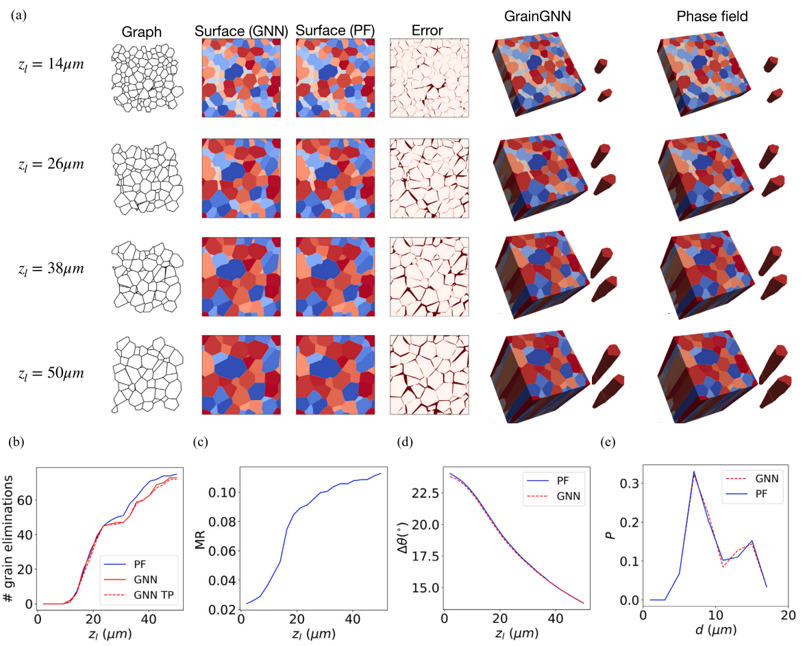
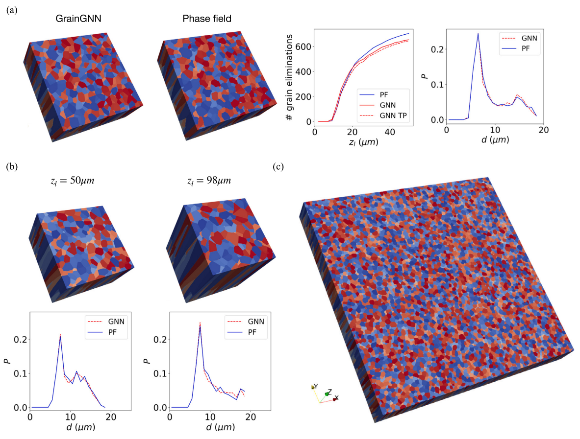
In the paper, the trained models are validated by comparing the predicted 3D field data with the high-fidelity data. We choose a phase field (PF) solver as the method to generate high-fidelity data. The codes can be found here https://github.com/YigongQin/cuPF. Under the folder rawdat_PF/, we provide two compressed PF data. One is of domain size (40um, 40um, 50um), and the other is of domain size (120um, 120um, 50um). To compare the GrainGNN results and PF results, and reproduce the results reported in the paper, follow the steps below.

Steps

For the domain size (40um, 40um, 50um):

Decompress the phase field data to .h5 file

gzip -d rawdat_PF/40_40/Epita_grains118_nodes236_frames120_G1.904_Rmax0.558_seed10020_Mt36920_train0_test1_rank0.h5.gz

Extract phase field data and create the graph for t=0

# specify the seed number, domain size with `--lxd`, raw data folder, and the output folder for graphs
python3 graph_trajectory.py --mode=test --rawdat_dir=./rawdat_PF/40_40/ --seed=10020 --lxd=40 --save_dir=./graphs/40_40/

After this step, you should get the files seed10020_G1.904_R0.558_span6.pkl and traj10020.pkl in graphs/40_40/. You can verify them with the files given in the repo.

Evolve the graph and get image results
```
# specify the folder of the graph data (--truth_dir) and seed number
python3 test.py --truth_dir=./graphs/40_40/ --seed=10020
```
After this step, you should get the plots for quantities of interest (QoIs) and image comparison for the last layer of grain structure. Compare the generated images with the Fig.8 of the paper

Similarly for the domain of (120um, 120um, 50um):

gzip -d rawdat_PF/120_120/Epita_grains1043_nodes2086_frames120_lxd120.000008_G10.000_Rmax2.000_UC20.000_seed0_Mt10300_rank0.h5.gz
python3 graph_trajectory.py --mode=test --rawdat_dir=./rawdat_PF/120_120/ --seed=0 --lxd=120 --save_dir=./graphs/120_120/
python3 test.py --truth_dir=./graphs/120_120/ --seed=0

Results correspond to Fig.11(a) of the paper

Numbers to check

case	error of last layer	grain event accuracy
/graphs/40_40/seed10020*	0.11	72/75
/graphs/120_120/seed0*	0.18	644/704

Inference the models only

The accuracy of the model under various thermal and grain configurations is discussed in the paper. If you are interested in the same material -- stainless steel 316L, and a similar range of thermal conditions, you can choose to run GrainGNN inference without having the high-fidelity data:

# specify thermal parameters (`G,R`), domain size `lxd`, and a seed number
python3 graph_trajectory.py --mode=generate --seed=1 --lxd=40 --save_dir=./graphs/40_40/ --G=10 --R=2
python3 test.py --truth_dir=./graphs/40_40/ --seed=1 --no-compare

Explore more arguments in graph_trajectory.py for more configuration, such as changing the grain size and orientation distributions with --size, --orien

Train models with the same phase field data (and extracted graphs) used in the paper

The graph pairs used for training can be downloaded here: https://drive.google.com/file/d/19uNh7XwHWMhF4PGLFcD-VM5YvYXBpHV_/view?usp=sharing
Decompress the file and optionally change the training parameters in the parameters.py

gzip dataset_train.pkl.gz
python3 train.py --model_type=regressor --model_id=0 --device=cuda
python3 train.py --model_type=classifier --model_id=1 --device=cuda

Log files of the training process are provided in model/ folder. The training curves can be found in the paper.

Create a new training dataset

The size of the full phase field training data is very large. We are figuring out ways to share the raw phase field data. Try generating new phase field data using codes here https://github.com/YigongQin/cuPF
To extract graph pairs from a PF .h5 file for training:

python3 graph_trajectory.py --mode=train --rawdat_dir=./rawdat_PF/40_40/ --seed=10020 --lxd=40 --save_dir=./graphs/40_40/

Then use create_datasets.py to combine graphs extracted from different PF files.

YigongQin/GrainGraphNN