The self-adapting mixture prior (SAMprior) package is designed to enhance the effectiveness and practicality of clinical trials by leveraging historical information or real-world data [1]. The package incorporate historical data into a new trial using an informative prior constructed based on historical data while mixing a non-informative prior to enhance the robustness of information borrowing. It utilizes a data-driven way to determine a self-adapting mixture weight that dynamically favors the informative (non-informative) prior component when there is little (substantial) evidence of prior-data conflict. Operating characteristics are evaluated and compared to the robust Meta-Analytic-Predictive (rMAP) prior [2], which assigns a fixed weight of 0.5.
To install the package:
install.packages('devtools')
devtools::install_github("pengyang0411/SAMprior")Consider a randomized clinical trial to compare a treatment with a control in patients with ankylosing spondylitis. The primary efficacy endpoint is binary, indicating whether a patient achieves 20% improvement at week six according to the Assessment of SpondyloArthritis International Society criteria [3]. Nine historical data available to the control were used to construct the MAP prior:
| study | n | r |
|---|---|---|
| Baeten (2013) | 6 | 1 |
| Deodhar (2016) | 122 | 35 |
| Deodhar (2019) | 104 | 31 |
| Erdes (2019) | 23 | 10 |
| Huang (2019) | 153 | 56 |
| Kivitz (2018) | 117 | 55 |
| Pavelka (2017) | 76 | 28 |
| Sieper (2017) | 74 | 21 |
| Van der Heijde (2018) | 87 | 35 |
SAM prior is constructed by mixing an informative prior SAM_weight
function to achieve the degree of prior-data conflict [1]. The following
sections describe how to construct SAM prior in details.
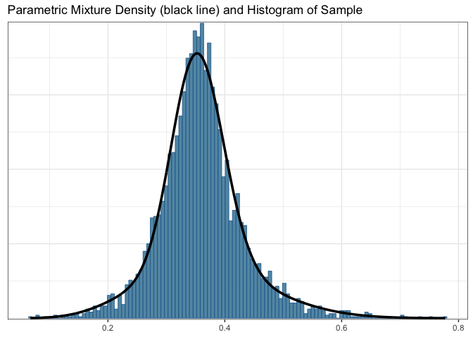
To construct informative priors based on the aforementioned nine
historical data, we apply gMAP function from RBesT to perform
meta-analysis. This informative prior results in a representative form
from a large MCMC samples, and it can be converted to a parametric
representation with the automixfit function using
expectation-maximization (EM) algorithm [4]. This informative prior is
also called MAP prior.
# load R packages
library(ggplot2)
theme_set(theme_bw()) # sets up plotting theme
set.seed(22)
map_ASAS20 <- gMAP(cbind(r, n-r) ~ 1 | study,
                   family = binomial,
                   data = ASAS20,
                   tau.dist = "HalfNormal",
                   tau.prior = 1,
                   beta.prior = 2)
## Assuming default prior location for beta: 0
map_automix <- automixfit(map_ASAS20)
map_automix
## EM for Beta Mixture Model
## Log-Likelihood = 5005.173
##
## Univariate beta mixture
## Mixture Components:
## comp1 comp2
## w 0.6347375 0.3652625
## a 42.5097011 7.1944569
## b 77.2077293 12.3741342
plot(map_automix)$mixThe resulting MAP prior is approximated by a mixture of conjugate priors,
given by
Let
The SAM prior uses the likelihood ratio test (LRT) statistics R to quantify the degree of prior-data conflict and determine the extent of information borrowing.
where P(D|⋅) denotes the likelihood function. An alternative Bayesian choice is the posterior probability ratio (PPR):
where
The SAM prior, denoted as
where the mixture weight
As the level of prior-data conflict increases, the likelihood ratio
To calculate mixture weight SAM_weight in SAMprior as follows:
n <- 35; r = 10
wSAM <- SAM_weight(if.prior = map_automix,
                   delta = 0.2,
                   n = n, r = r)
cat('SAM weight: ', wSAM)
## SAM weight: 0.7900602
The default method to calculate
wSAM <- SAM_weight(if.prior = map_automix,
                   delta = 0.2,
                   method.w = 'PPR',
                   prior.odds = 3/7,
                   n = n, r = r)
cat('SAM weight: ', wSAM)
## SAM weight: 0.6172732
The prior.odds indicates the prior probability of prior.odds = 3/7), the prior
information favors the presence prior-data conflict and it results in a
decreased mixture weight.
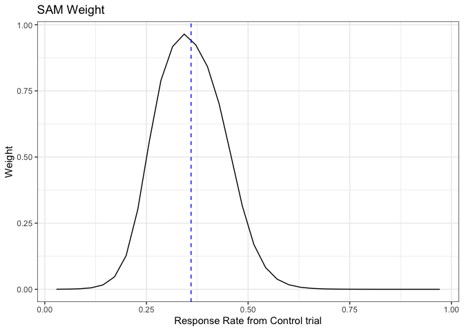
When historical information is congruent with the current control arm,
SAM weight reaches to the highest peak. As the level of prior-data
conflict increases, SAM weight decreases. This demonstrates that SAM
prior is data-driven and self-adapting, favoring the informative
(non-informative) prior component when there is little (substantial)
evidence of prior-data conflict.

To construct the SAM prior, we mix the derived informative prior SAM_prior function in SAMprior as follows:
SAM.prior <- SAM_prior(if.prior = map_automix,
                       nf.prior = mixbeta(nf.prior = c(1,1,1)),
                       weight = wSAM)
SAM.prior
## Univariate beta mixture
## Mixture Components:
## comp1 comp2 nf.prior
## w 0.3918065 0.2254667 0.3827268
## a 42.5097011 7.1944569 1.0000000
## b 77.2077293 12.3741342 1.0000000
where the non-informative prior
Finally, we present an example of how to make a final decision on
whether the treatment is superior or inferior to a standard control once
the trial has been completed and data has been collected. This step can
be accomplished using the postmix function from RBesT, as shown
below:
## Sample size and number of responses for treatment arm
n_t <- 70; x_t <- 22

## first obtain posterior distributions...
post_SAM <- postmix(priormix = SAM.prior,         ## SAM Prior
                    r = r,   n = n)
post_trt <- postmix(priormix = mixbeta(c(1,1,1)), ## Non-informative prior
                    r = x_t, n = n_t)

## Define the decision function
decision = decision2S(0.95, 0, lower.tail=FALSE)

## Decision-making
decision(post_trt, post_SAM)
## [1] 0
Peng Yang (py11@rice.edu)
[1] Yang P. et al., Biometrics, 2023; 00, 1–12. https://doi.org/10.1111/biom.13927
[2] Schmidli H. et al., Biometrics, 2014; 70(4):1023-1032.
[3] Baeten D. et al., The Lancet, 2013; (382), 9906, p 1705.
[4] Neuenschwander B. et al., Clin Trials, 2010; 7(1):5-18.
