pg-gan

This software can be used to create realistic simulated data that matches real population genetic data. It implements a GAN-based algorithm (Generative Adversarial Network) described in the pre-print Automatic inference of demographic parameters using Generative Adversarial Networks.

Python 3.6 (or later) is required, along with the following libraries (these exact versions are likely not necessary, but should be similar):

msprime==0.7.4
numpy==1.17.2
tensorflow==2.2.0

See the msprime documentation and tensorflow pip guide for installation instructions.

Dependencies for pre-processing real data (not needed to try out the first two simulation command lines below):

h5py==2.10.0

Link: HDF5 for Python

Dependencies for creating summary statistic plots:

allel==1.2.1

Link: scikit-allel

Demographic models

There are currently six demographic models implemented in pg-gan (see below for information about adding your own model). Use the -m flag to specify the model (required parameter).

CONST (command line const): constant population size (Ne)
IM (command line im): isolation-with-migration (two-population model)
EXP (command line exp): one-population exponential growth model
OOA2 (command line ooa2): Out-of-Africa model with two populations (e.g. YRI/CEU or YRI/CHB)
POST (command line post_ooa): post Out-of-Africa split with two populations (e.g. CEU/CHB)
OOA3 (command line ooa3): three-population Out-of-Africa model (e.g. YRI/CEU/CHB), as specified in Gutenkunst et al 2009 and implemented in stdpopsim.

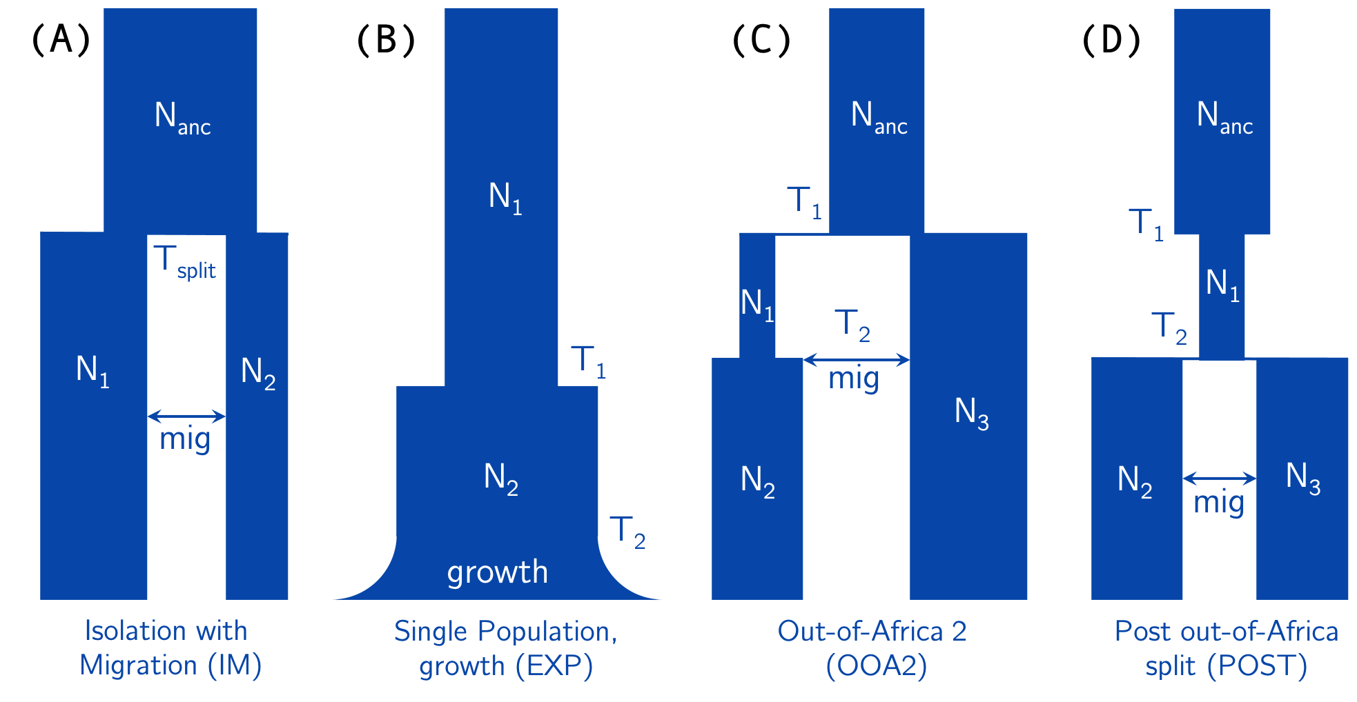
See the diagram below for the parameters of IM, EXP, OOA2, and POST. Mutation (mut) and recombination (reco) can also be added to the list of parameters to infer.

Simulated training data

Below are two examples with simulated training data. In this case the training data is simulated under fixed parameter values (see the manuscript link above for details). Then pg-gan attempts to infer these "true" values.

Note that all output is printed to stdout, including current parameter estimates and GAN confusion. If you save this output to a file, it can then be read in by the summary statistic visualization program.

Toy example with simulated training data. -m im means use the IM model (isolation-with-migration) and -p is used to specify the parameters to infer (six here). -t is the "toy" flag, which will run the method without discriminator pre-training and then for two iterations only. It should take about 5 min with a GPU.

python3 pg_gan.py -m im -p N1,N2,N_anc,T_split,reco,mig -t

The last two lines of the output contain:

A list of all parameter sets throughout training. The last set is used as the final inference. For example in this case the parameters values are: [7.118372774235415e-08, 4762.012023755695, 12480.088492825884, 0.061209667268172285, 1614.4605003581084, 20970.075968181205], although yours will be different.
A list of all generator loss values throughout training. In this case I obtained [6.124907, 4.915148, 2.7859032] (loss at the beginning as well as the loss after the two iterations). This is good since the loss is decreasing as the generator starts to move toward more realistic parameters (although two iterations will not get very far).

Same example above but without the "toy" flag. This will take several hours to run (likely 5-6 with a GPU, more without one).

python3 pg_gan.py -m im -p N1,N2,N_anc,T_split,reco,mig

Real training data

Below is a tutorial that explains how to run pg-gan on the 1000 Genomes data. Modifications may be needed for other data, but the process should generally be similar.

Note: this tutorial will require bcftools.

Download the Phase 3 ALL VCF files from the 1000 Genomes Project for chromosomes 1-22. Also download the accessibility mask 20120824_strict_mask.bed.
Identify a set of samples for the population of interest. Here we will use CHB, and a sample file is provided above in prep_data/CHB_gan.txt. When using more than one population, make sure the samples are sorted by population (and currently equal numbers from each population are needed). Data from all populations eventually needs to end up in the same VCF file and then the same HDF5 file.
Create a list of VCF files to use as training data. Here we will use chromosomes 1-22 from CHB, and the list of files is provided in prep_data/CHB_filelist.txt.
Prepare the VCF files using bcftools. This will remove non-segregating sites and multi-allelic sites, as well as retain our desired samples and concatenate chromosomes 1-22 into one VCF file. To do all these operations, use the file prep_data/prep_vcf.sh.

sh prep_data/prep_vcf.sh

Convert this final VCF file into HDF5 format:

python3 vcf2hdf5.py -i CHB.phase3_shapeit2_mvncall_integrated_v5a.20130502.genotypes.vcf.gz -o CHB.phase3_shapeit2_mvncall_integrated_v5a.20130502.genotypes.h5

Finally, run pg-gan on the data using (for example) a 5-parameter exponential growth model.

python3 pg_gan.py -m exp -p N1,N2,growth,T1,T2 -d CHB.phase3_shapeit2_mvncall_integrated_v5a.20130502.genotypes.h5 -b 20120824_strict_mask.bed

Use -r (optional) to specify a folder with recombination map files for each chromosome (for example -r genetic_map/). This will cause the generator to sample from this recombination rate distribution when creating simulated data. See the start of file genetic_map_GRCh37_chr1.txt below for the format of the recombination map files.

Chromosome      Position(bp)    Rate(cM/Mb)     Map(cM)
chr1    55550   2.981822        0.000000
chr1    82571   2.082414        0.080572
chr1    88169   2.081358        0.092229
chr1    254996  3.354927        0.439456
...

Visualizing summary statistics

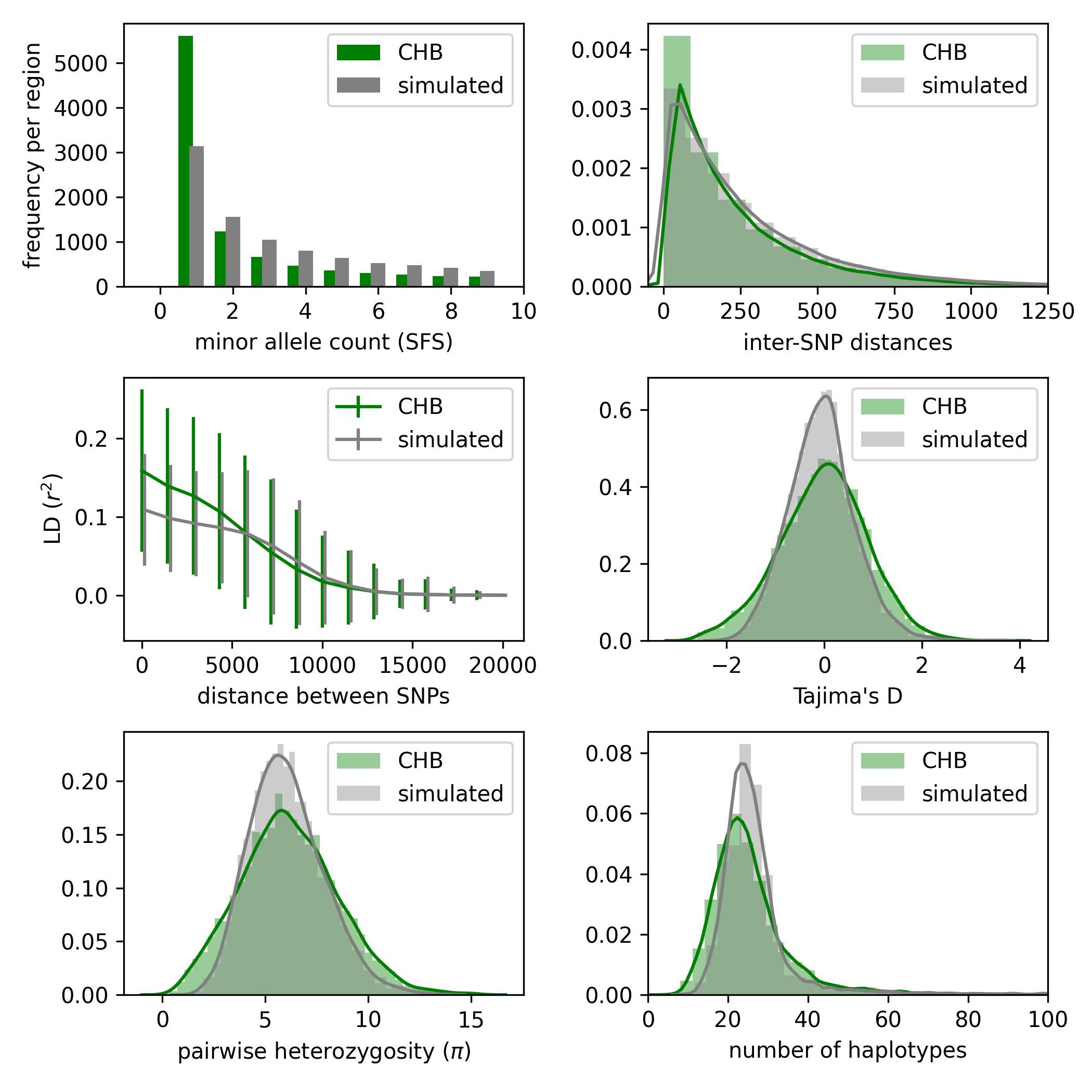
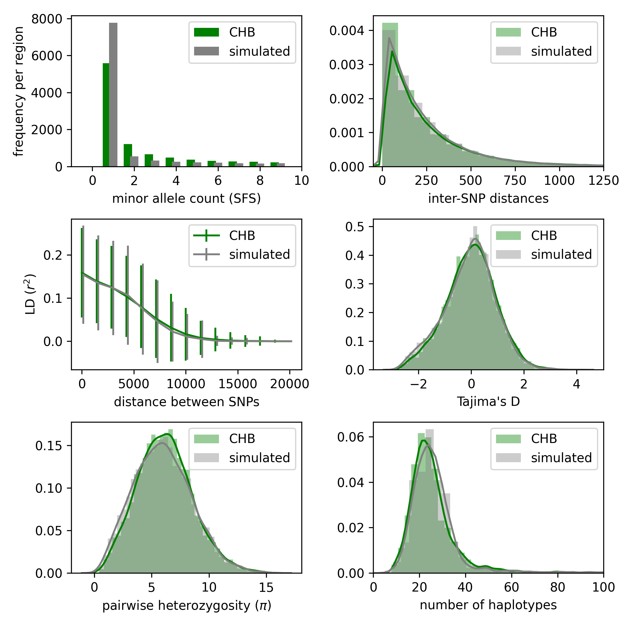
After running pg-gan, the resulting parameters can be used to simulate data, which can then be compared to the real data via summary statistics. For example, to reproduce (roughly) the figures below, run the following commands:

python3 pg_gan.py -m const -p Ne -d CHB.phase3_shapeit2_mvncall_integrated_v5a.20130502.genotypes.h5 -b 20120824_strict_mask.bed -r genetic_map/ > chb_const.out

python3 summary_stats.py chb_const.out chb_const.png -m const -p Ne -d CHB.phase3_shapeit2_mvncall_integrated_v5a.20130502.genotypes.h5 -b 20120824_strict_mask.bed -r genetic_map/

The second command with summary_stats.py generates a plot (similar to the one below). The input file is chb_const.out and the output file is chb_const.png, but the rest of the command line arguments are the same as pg-gan.

Here is another example with the EXP model instead of CONST:

python3 pg_gan.py -m exp -p N1,N2,growth,T1,T2 -d CHB.phase3_shapeit2_mvncall_integrated_v5a.20130502.genotypes.h5 -b 20120824_strict_mask.bed -r genetic_map/ > chb_exp.out

python3 summary_stats.py chb_exp.out chb_exp.png -m exp -p N1,N2,growth,T1,T2 -d CHB.phase3_shapeit2_mvncall_integrated_v5a.20130502.genotypes.h5 -b 20120824_strict_mask.bed -r genetic_map/

Creating your own models

You can add your own demographic models to pg-gan, as long as they are implemented in msprime. Right now new models must be added as functions to simulation.py. Each function should return an msprime tree sequence. Here is an example for the CONST model. The params should match those in the util.py file (although more can be added as needed), and the sample_sizes should be a list of integers (with length matching the number of populations). The other parameters of the function can be ignored unless the user wants to customize them.

def simulate_const(params, sample_sizes, L, seed, prior=[], weights=[]):
    assert len(sample_sizes) == 1

    # sample reco or use value
    if prior != []:
        reco = draw_background_rate_from_prior(prior, weights)
    else:
        reco = params.reco.value

    # simulate data
    ts = msprime.simulate(sample_size=sum(sample_sizes), Ne=params.Ne.value, \
        length=L, mutation_rate=params.mut.value, recombination_rate=reco, \
        random_seed = seed)

    return ts

After adding this function, register it in the process_opts function of pg_gan.py as a new option. For one-population models use the OnePopModel discriminator, for two-population models use TwoPopModel, and for three-population models use ThreePopModel. The sample_sizes variable should be a list of integers matching the number of haplotypes in each population.

if opts.model == 'const':
    sample_sizes = [198]
    discriminator = discriminators.OnePopModel()
    simulator = simulation.simulate_const

General notes

We recommend running pg-gan 10 times, then selecting the run with the lowest discriminator accuracy on generated data (i.e. which run produces data that is most easily confused for real data). If any runs result in a discriminator that always predicts the same class (either all real or all simulated), reject the run.

pg-gan is under active development. Please reach out to Sara Mathieson (smathieson [at] haverford [dot] edu) with any questions.