Persistence B-Spline Grids: Stable Vector Representation of Persistence Diagrams

This is an implementation of Persistence B-Spline Grids on Matlab and Python3.

Requirements

To run the code, there are some requirements:

pip install numpy matplotlib scikit-tda tqdm seaborn pandas scikit-learn

Jupyter is required to run the .ipynb. The PB_code folder should be uploaded.

Example 1 (toydata)

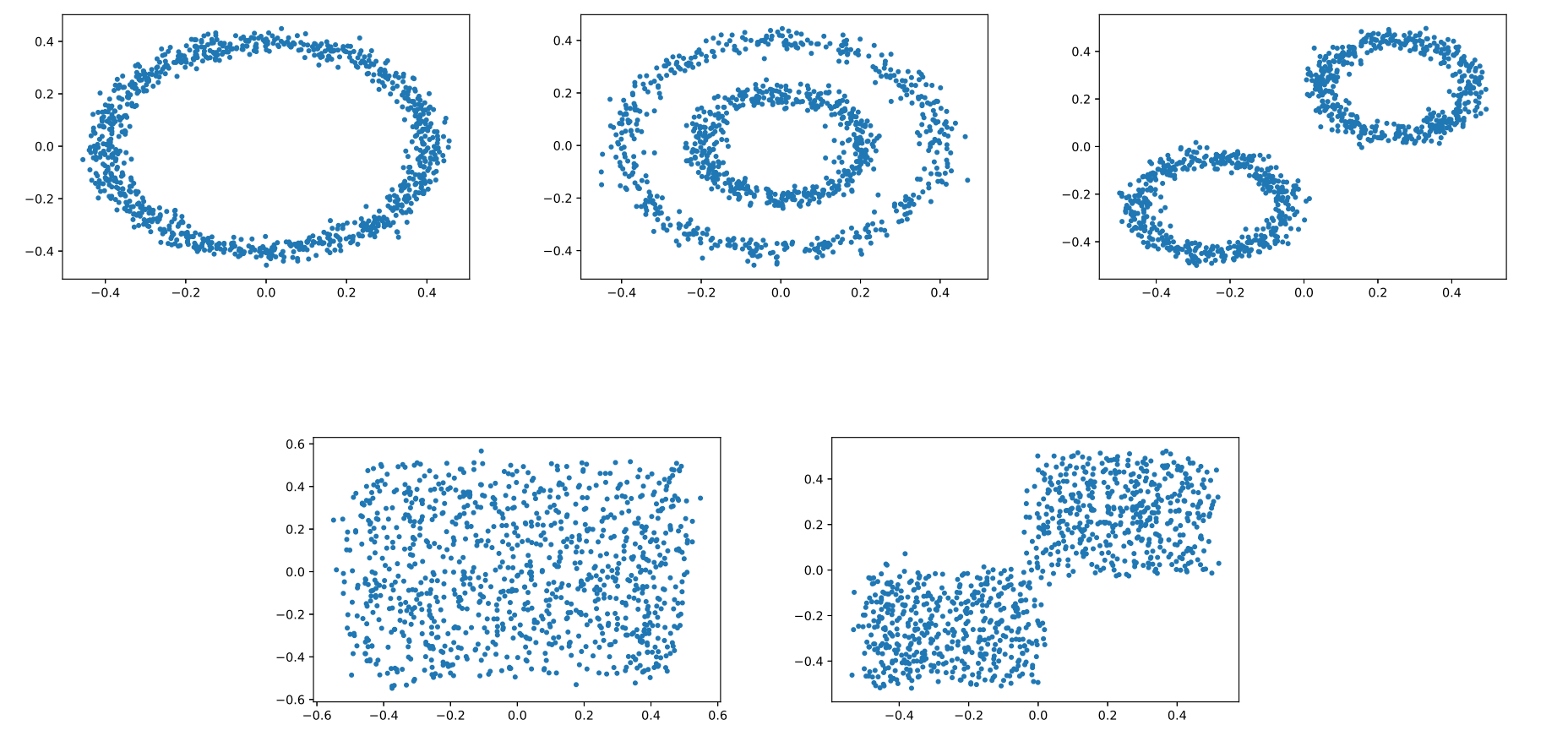
An example of toydata is provided. It is a simple synthetic toy data set that contains a circle with its radius 0.4, two concentric circles with their radii 0.2 and 0.4, respectively, two disjoint circles with both their radii 0.2, a cluster of points sampled at random in the normal square, and two clusters of points sampled at random separately in two squares with edge length 0,5. All data are sampled in the range of [−0.5, 0.5]^2 on the 2D plane (shown as follows).

Follow the procedures:

Run PD_toydata.ipynb to generate PDs in PD_toydata folder.
Run Matlab code main_toydata.m to compute PBs. The results are saved in PB_toydata folder.
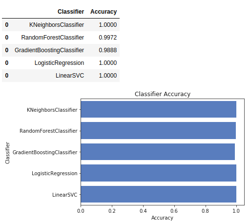
Run classify_toydata.ipynb and obtain the accuracy of classification shown like the following figure.

Example 2 (3D dynamical system)

Because computing PDs takes several hours, the PD dataset was computed in advance, and was saved in PD_dynamic3d folder. If you wanted to test the algorithm directly, you could skip to step3.

Follow the procedures:

Run dynamic_3d.m in data folder to generate original data.
Run PD_dynamic.ipynb to generate PDs in PD_dynamic3d folder.
Run Matlab code main_dynamic3d.m to compute PBs. The results are saved in PB_dynamic3d folder.
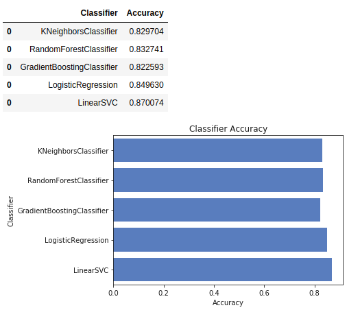
Run classify_dynamic3d.ipynb and obtain the accuracy of classification shown like the following figure.

Example 3 (Randomly-generate PD)

The dataset of randomly-generated PDs was formed to evaluate the method PB: (1) the classification performance of random PDs with randomly marked label to dispel doubts of over-performance, and (2) performance on two designed randomly generated PD dataset with different distribution and density of long-persistence points to explain which features of PDs PB can capture.

Follow the procedure:

Run randomPD_test.m in data folder to generate random PDs with different distribution and density. (Randomly-generated PDs in (1) are given in ./data/randomPD folder.)
Run RandomPD2PB.m to compute PBs. Data is in PB_ClassifyrandomPD folder and PB_rPD_Evaluation folder.
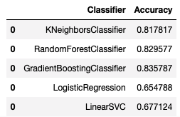
Run classify_randomPD.ipynb to obtain the classification accuracy in Test (1) and run classifier_rPD_Evaluation.ipynb to obtain the results of Test (2).

Experiment in Appendix

Example 4 (PC)

original data are in Google Drive. Unzip to data/PC_train,
Run PD_pc.ipynb to generate PDs in PD_pc folder. We provide them in Google Drive.
Run Matlab code main_pc.m to compute PB of PD. The results are saved in PB_pc folder.
Run classify_pc.ipynb and see the accuracy of classification.

Relationship between stable coefficient and the iteration of LSPIA

The randomly-generated PD dataset is in ./data/PD4theorem folder.

Run iteration_test.m in data folder to generated PBs.
Run ThmCoefTest.m to generate iteraion-ratio figure.