FVTool: Finite volume toolbox for Matlab

Tiny Documents 📘.

This is a finite volume (toy) toolbox for chemical/petroleum engineers. Right now, it can solve a transient convection-diffusion equation with variable velocity field/diffusion coefficients. The discretization schemes include:

central difference diffusion term
central difference convection term
upwind convection term
TVD convection term with various flux limiters
transient term
Dirichlet, Neumann, Robin, and periodic boundary conditions

Which equation do you solve?

You can solve the following PDE (or a subset of it):

with the following boundary conditions:

Believe it or not, the above equations describe the majority of the transport phenomena in chemical and petroleum engineering and similar fields.

How to start

Download the package, start matlab, and run FVToolStartUp

Inspiration

I started writing this tool after playing with FiPy, an amazing python-based finite volume solver. This matlab solver is not a clone, and indeed very limited compared to FiPy. I wrote it to have a very handy tool for testing new ideas (new mathematical models) by solving them in 1D uniform Cartesian grids. Then I extended the code to

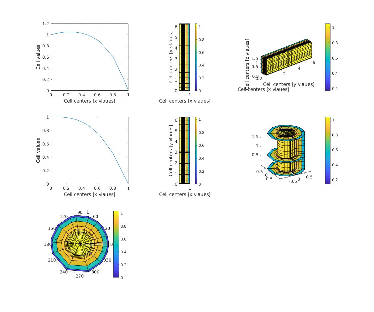
1D axisymmetric (radial)
2D radial (r, theta)
2D Cartesian
3D Cartesian
2D axisymmetric (cylindrical, r, z)
3D cylindrical (r, theta, z)

I have overloaded some of the matlab operators to simplify the switch from 1D codes to 2D and 3D.

A simple example

You can solve a diffusion equation, i.e., $ \nabla. (-D \nabla \phi) = 0 $ by running the following code in Matlab:

clc
L = 50;  % domain length
Nx = 20; % number of cells
m = createMesh1D(Nx, L);
BC = createBC(m); % all Neumann boundary condition structure
BC.left.a(:) = 0; BC.left.b(:)=1; BC.left.c(:)=1; % Dirichlet for the left boundary
BC.right.a(:) = 0; BC.right.b(:)=1; BC.right.c(:)=0; % right boundary
D_val = 1; % value of the diffusion coefficient
D = createCellVariable(m, D_val); % assign the diffusion coefficient to the cells
D_face = harmonicMean(D); % calculate harmonic average of the diffusion coef on the cell faces
Mdiff = diffusionTerm(D_face); % matrix of coefficients for the diffusion term
[Mbc, RHSbc] = boundaryCondition(BC); % matrix of coefficients and RHS vector for the BC
M = Mdiff + Mbc; % matrix of coefficients for the PDE
c = solvePDE(m,M, RHSbc); % send M and RHS to the solver
visualizeCells(c); % visualize the results

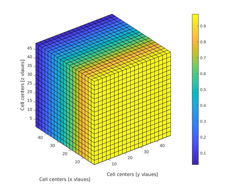
change the third line to m = createMesh2D(Nx,Nx, L,L); or m = createMesh3D(Nx,Nx,Nx, L,L,L); and see the outcome for yourself.

Examples

There are a few simple examples in the Tutorial folder. You can also find a few more advanced examples (water injection into a heterogeneous oil field, two nonlinear PDEs, coupled fully implicit solution) in the Advanced folder.

Documents

Find some preliminary documents here.

But Matlab is not a free software?

You can use the code in octave. The new (object oriented) version of the code works in Octave 4.0 (with the new classdef function).
I've re-written the code in Julia. It works fine, but the visualization on Windows OS has still some issues.

Questions and bug reports

You can ask your questions by creating a new issue here, or by writing a comment in my blog. You can also ask your question in the Matlab file exchange page of this code. I truly appreciate your feedback and/or contribution.

How to cite:

If you have used the package in your work and you find it usefull, please cite it as:

@misc{ali_akbar_eftekhari_2015_32745,
  author       = {Ali Akbar Eftekhari and Kai Schüller and Ferran Brosa Planella and Martinus Werts and Behzad Hosseinzadeh},
  title        = {FVTool: a finite volume toolbox for Matlab},
  month        = oct,
  year         = 2015,
  doi          = {10.5281/zenodo.32745},
  url          = {https://doi.org/10.5281/zenodo.32745}
}

I will also appreciate it if you write me a couple of lines about how you have used it in your research. It encourages me to maintain the code.

ZhouChuanyou/FVTool