- Learn how to install Python packages.
- Get familiar with three popular Python packages for working with, analyzing, and plotting data.
- Getting set up
- Installing Python packages
- Learning how to use the packages
- The exercise
- Acknowledgments
- License
At this point, you should have (1) an account on Github and (2) been introduced to the very basics of Git.
-
Login to your Github account.
-
Fork this repository, by clicking the 'Fork' button on the upper right of the page.
After a few seconds, you should be looking at your copy of the repo in your own Github account.
-
Click the 'Clone or download' button, and copy the URL of the repo via the 'copy to clipboard' button.
-
In your terminal, navigate to where you want to keep this repo (you can always move it later, so just your home directory is fine). Then type:
$ git clone the-url-you-just-copiedand hit enter to clone the repository. Make sure you are cloning your fork of this repo.
-
Next,
cdinto the directory:$ cd the-name-of-directory-you-just-cloned -
At this point, you should be in your own local copy of the repository.
-
As you work on the exercise below, be sure to frequently
addandcommityour work andpushchanges to the remote copy of the repo hosted on GitHub. Don't enter these commands now; this is just to jog your memory:$ # Do some work $ git add file-you-worked-on.py $ git commit $ git push origin master
For this exercise, we will be using three popular Python packages:
- pandas
- pandas is a great package for easily parsing, manipulating, and analyzing tabular data.
- matplotlib
- matplotlib is the most popular Python package for visualizing (plotting) data.
- SciPy
- SciPy is Python package for, well, science!
pandas, matplotlib, and scipy are not built-in modules, like sys, os,
and re.
Before we use them as modules, we need to install them from external packages.
How you install Python packages will depend on the Python installation you are
using.
If you are using Python installed with
Anaconda
or
Miniconda
you will use the conda tool to install packages.
Otherwise, you will use the pip module to install packages.
Not sure what installation of Python you are using? No problem, we can check. Run this command on the command line to see the path to the Python you are using:
$ which python3
If python3 is inside an anaconda or miniconda directory
(e.g., /home/jamie/miniconda3/bin/python3),
you will use conda to install packages.
If so, you can run:
$ which conda
and that should confirm that conda is available in
the same directory as python3
(e.g., /home/jamie/miniconda3/bin/conda).
If python3 is NOT inside an anaconda or miniconda directory
(e.g., /usr/bin/python3),
you will use pip to install packages.
If you are using a "normal" installation of Python (not anaconda/miniconda),
you can use the pip module to install packages.
To install the pandas, matplotlib, and scipy packages, run this command
at the command line:
$ python3 -m pip install scipy matplotlib pandas
If you are using anaconda or miniconda, you can use the conda tool to install
the pandas, matplotlib, and scipy packages:
$ conda install scipy matplotlib pandas
To verify that the packages were installed correctly, fire-up the Python interpreter:
$ python3
And try importing pandas and matplotlib:
>>> import pandas
>>> import matplotlib
>>> import scipy
If you get an error when trying to import a package, then it is not installed correctly.
We will only scratch the surface of what these packages are capable of. However, all three are very well documented, so you can refer to their online documentation to take these tools further.
Let's open our Python interpreter and play around with pandas a bit.
Enter the lines below in the interpreter to import the pandas module and read
data from a CSV file into a DataFrame object:
>>> import pandas as pd
>>> dataframe = pd.read_csv("iris.csv")
>>> type(dataframe)
>>> print(dataframe)
The output from the print statement should look like:
     sepal_length_cm  sepal_width_cm  petal_length_cm  petal_width_cm         species
0                5.1             3.5              1.4             0.2     Iris_setosa
1                4.9             3.0              1.4             0.2     Iris_setosa
2                4.7             3.2              1.3             0.2     Iris_setosa
3                4.6             3.1              1.5             0.2     Iris_setosa
4                5.0             3.6              1.4             0.2     Iris_setosa
..               ...             ...              ...             ...             ...
145              6.7             3.0              5.2             2.3  Iris_virginica
146              6.3             2.5              5.0             1.9  Iris_virginica
147              6.5             3.0              5.2             2.0  Iris_virginica
148              6.2             3.4              5.4             2.3  Iris_virginica
149              5.9             3.0              5.1             1.8  Iris_virginica
These are morphological data from three species of Iris; you can
learn more about these data here.
Notice, when we imported pandas we gave it a shorter name pd.
This is common practice with some Python packages.
We will adhere to this practice, because you are likely to see it
when searching the interweb for help with pandas and matplotlib.
Next, let's learn the basics of how to access the data in a pandas
DataFrame.
There are two ways to access columns of a data frame. One is to use the "dot" syntax to access them as attributes of the object:
>>> dataframe.sepal_length_cmThe other is to use dict-like syntax to access them using
the column header as a key:
>>> dataframe["sepal_length_cm"]Both ways will get the same result:
0      5.1
1      4.9
2      4.7
3      4.6
4      5.0
      ...
145    6.7
146    6.3
147    6.5
148    6.2
149    5.9
Name: sepal_length_cm, Length: 150, dtype: float64
We can use iloc (short for index location) to access the first row of the
data frame:
dataframe.iloc[0]sepal_length_cm 5.1
sepal_width_cm 3.5
petal_length_cm 1.4
petal_width_cm 0.2
species Iris_setosa
Name: 0, dtype: object
To access the first 3 rows we can use:
dataframe.iloc[0:3] sepal_length_cm sepal_width_cm petal_length_cm petal_width_cm species
0 5.1 3.5 1.4 0.2 Iris_setosa
1 4.9 3.0 1.4 0.2 Iris_setosa
2 4.7 3.2 1.3 0.2 Iris_setosa
To get the value at first row of first column, use:
>>> dataframe.iloc[0, 0]
5.1
To get the values at first three rows of first column, you can:
>>> dataframe.iloc[0:3, 0]
0    5.1
1    4.9
2    4.7
Name: sepal_length_cm, dtype: float64
We can get the same result of the last line using:
>>> dataframe.sepal_length_cm[0:3]Or:
>>> dataframe["sepal_length_cm"][0:3]Now, let's learn how to filter out subsets of the data frame. First, let's get a new data frame that only contains plants with flower petals longer than 5.9 cm:
>>> long_flowers = dataframe[dataframe.petal_length_cm > 5.9]
>>> print(long_flowers)
sepal_length_cm sepal_width_cm petal_length_cm petal_width_cm species
100 6.3 3.3 6.0 2.5 Iris_virginica
105 7.6 3.0 6.6 2.1 Iris_virginica
107 7.3 2.9 6.3 1.8 Iris_virginica
109 7.2 3.6 6.1 2.5 Iris_virginica
117 7.7 3.8 6.7 2.2 Iris_virginica
118 7.7 2.6 6.9 2.3 Iris_virginica
122 7.7 2.8 6.7 2.0 Iris_virginica
125 7.2 3.2 6.0 1.8 Iris_virginica
130 7.4 2.8 6.1 1.9 Iris_virginica
131 7.9 3.8 6.4 2.0 Iris_virginica
135 7.7 3.0 6.1 2.3 Iris_virginica
Next, let's get a new data frame with data for one Iris species only:
>>> versicolor = dataframe[dataframe.species == "Iris_versicolor"]
>>> print(versicolor)
sepal_length_cm sepal_width_cm petal_length_cm petal_width_cm species
50 7.0 3.2 4.7 1.4 Iris_versicolor
51 6.4 3.2 4.5 1.5 Iris_versicolor
52 6.9 3.1 4.9 1.5 Iris_versicolor
53 5.5 2.3 4.0 1.3 Iris_versicolor
54 6.5 2.8 4.6 1.5 Iris_versicolor
55 5.7 2.8 4.5 1.3 Iris_versicolor
56 6.3 3.3 4.7 1.6 Iris_versicolor
57 4.9 2.4 3.3 1.0 Iris_versicolor
58 6.6 2.9 4.6 1.3 Iris_versicolor
.
.
.
Next, let's learn the basics of plotting with matplotlib.
quit() your previous Python interpreter session and open
a new one:
$ python3
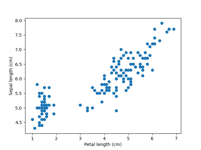
Import pandas and matplotlib, read the Iris data into a data frame, and
generate a simple scatter plot:
import pandas as pd
import matplotlib.pyplot as plt
dataframe = pd.read_csv("iris.csv")
plt.scatter(dataframe.petal_length_cm, dataframe.sepal_length_cm)
plt.xlabel("Petal length (cm)")
plt.ylabel("Sepal length (cm)")
plt.savefig("petal_v_sepal_length.png")
quit()
You should now have a file named petal_v_sepal_length.png in your current
directory.
If you open this PNG file it should look like:
Open your Python interpreter again:
$ python3
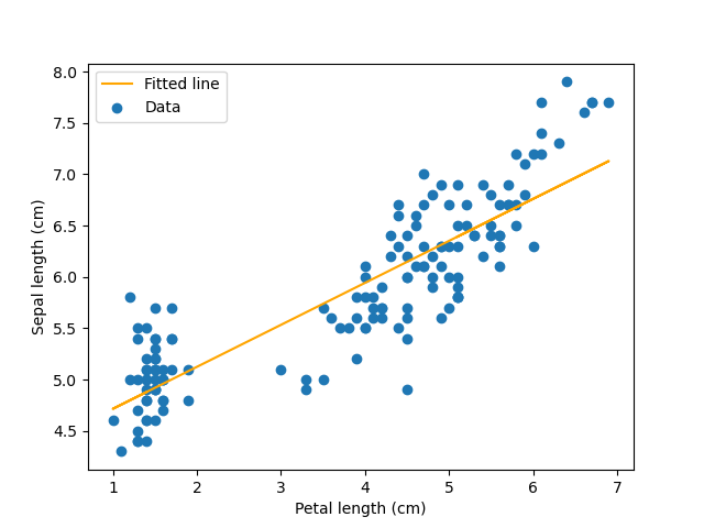
Below, we will import the stats module of scipy along with pandas and
matplotlib,
run a linear regression of sepal length against petal length,
and add the regression line to our plot:
import pandas as pd
import matplotlib.pyplot as plt
from scipy import stats
dataframe = pd.read_csv("iris.csv")
x = dataframe.petal_length_cm
y = dataframe.sepal_length_cm
regression = stats.linregress(x, y)
slope = regression.slope
intercept = regression.intercept
plt.scatter(x, y, label = 'Data')
plt.plot(x, slope * x + intercept, color = "orange", label = 'Fitted line')
plt.xlabel("Petal length (cm)")
plt.ylabel("Sepal length (cm)")
plt.legend()
plt.savefig("petal_v_sepal_length_regress.png")
quit()
You should now have another PNG file (petal_v_sepal_length_regress.png) that
looks like:
Write a Python script to perform the linear regression and create the plot we did above but for each of the three species of Iris separately. Use best practices when writing your script. For example:
- Make your code modular and reusable by breaking it up into functions.
- Use docstrings to document your script and functions.
- Write expressive code (e.g., use descriptive variable names).
- Make your script importable by using
if __name__ == '__main__'.
This work was made possible by funding provided to Jamie Oaks from the National Science Foundation (DEB 1656004).
This work is licensed under a Creative Commons Attribution 4.0 International License.


