This is a collection of MLflow project examples that you can directly run with mlflow CLI commands or directly using Python.
The goal is provide you with additional set of samples, focusing on machine learning and deep learning examples, to get you quickly started on MLFlow. In particular, I focus on Keras and borrow and extend examples from Francois Cholllet's book: Deep Learning with Python
This is a simple Keras neural network model with three layers, one input, one hidden,
and one output layer. It's a simple linear model: y=Mx. Given a random numbers of X values,
it learns to predict it's Y value, from a training set.
This Multi-layer Perceptron (MLP) for binary classification model's sources have been modified from this gist. You can use other network models from this gist in a similar fashion to experiment.
The arguments to run this simple MLP Keras network model are as follows:
--drop_rate: Optional argument with a default value is0.5.--input_dim: Input dimension. Default is20.--bs: dimension and size of the data. Default is(1000, 20)--output: Output to connected hidden layers. Default is64.--train_batch_size: Training batch size. Default is128--epochs: Number of epochs for training. Default is20.
To experiment different runs to evaluate metrics, you can alter the arguments, for example,
expand the size of network by providing more output to the hidden layers. Or you
may change the drop_rate or train_batch_size — all will alter the loss and
accuracy of the network model.
To run the current program with just python and yet log all metrics, use the following command:
python keras/keras_nn_model.py
python keras/keras_nn_model.py --output=128 --epochs=10
python keras/keras_dnn/main_nn.py --output=128 --epochs=10
It will log metrics and parameters in the mlruns directory.
Alternatively, you can run using the mlflow command.
mflow run . e -keras-nn-model
mlflow run . -e keras-nn-model -P drop_rate=0.3 -P output=128
The next two examples are from Deep Learning with Python. While the Jupyter notebooks can be found here, I have modified the code to tailor for use with MLflow. The description and experimentation remain the same, hence it fits well with using MLflow to experiment various capacity of networks layers and suggested parameters to evaluate the model.
This part comprises of code samples found in Chapter 3, Section 5 of Deep Learning with Python. The borrowed code from the book has been modularized and adjusted to work with MLflow, and it fits well since Francois suggests some experimentation parameters to tweak to see how the model metrics change.
Two-class classification, or binary classification, may be the most widely applied kind of machine learning problem. In this example, we will learn to classify movie reviews into "positive" reviews and "negative" reviews, just based on the text content of the reviews.
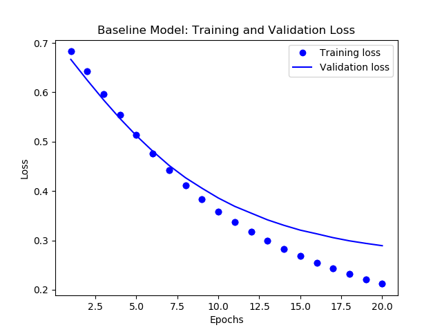
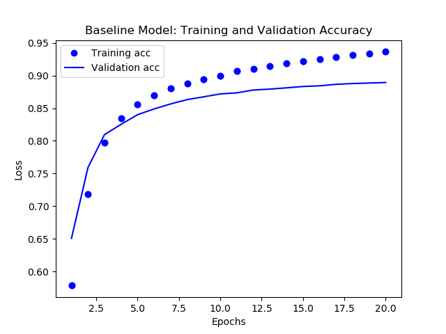
This example creates two types of models for you to work with. First, it creates a baseline model with default parameters:
- loss function as
rmstrop binary_crossentropyfor metrics- learning rate as 0.001
- a Keras neural network model with
- An input layer with input_shape (10000, )
- 1 hidden layer with output = 32
- 1 Output layer with output = 1
- All layers use
reluas an activation function except forsigmodthat is used in the final output layer.
- epochs = 20; batch_size=512
And the second model can me created for experimenting by changing any of the these parameters to measure the metrics:
- Use 2 or more hidden layers
- Use 4, 8, 12 or 16 epochs
- Try hidden layers with output 32, 64 or 128 and see if that affects the metrics
- Try to use the
mseloss function instead ofbinar_crossentropy.
In both cases, the model will create images for training and validation loss/accuracy images in the images directory
To run the current program with just python and default or supplied parameter and yet log all metrics, use the following command:
cd bckerasnn
python main_nn.py
To experiment different runs, with different parameters suggested above, and evaluate new metrics, you can alter the arguments. For example,
expand the size of network by providing more output to the hidden layers. Or you
may change the hidden_layers or epochs or loss function — all will alter the loss and
accuracy of the network model. For example,
python main_nn.py --hidden_laysers=3 --output=32 --epochs=30 --loss=mse
It will log metrics and parameters in the mlruns directory.
Alternatively, you can run using the mlflow command.
Note: mlflow run.. may take longer as it needs to create and setup an environment by and downloand and
installing dependency packages listed in conda.yml
mlflow run . -e binary-nn-model
mlflow run . -e binary-nn-model -P hidden_layers=3 -P output=32 -P epochs=30 -P loss=mse
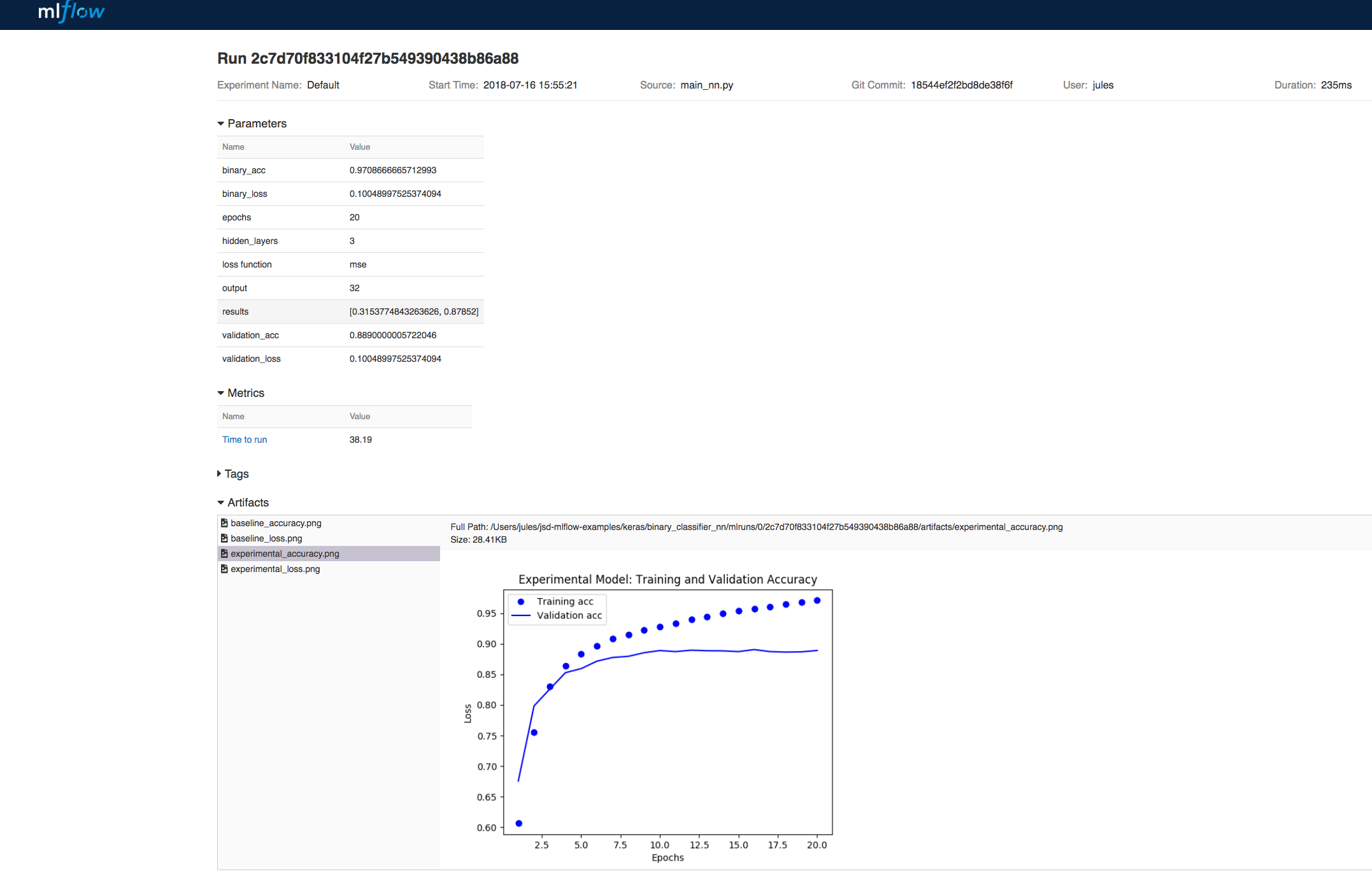
To view the output of either runs, launch the mlflow ui:
mlflow ui
These runs will not only log metrics for loss and accuracy but also log graphs generated from matplotlib for
perusal as part of visual artifacts.
Finally, you can run this in a Jupyter Notebook:
This contains the code samples found in Chapter 3, Section 5 of Deep Learning with Python.
In the above model we saw how to classify vector inputs into two mutually exclusive classes using a densely-connected neural network. But what happens when you have more than two classes?
In this section, we will build a network to classify Reuters newswires into 46 different mutually-exclusive topics. Since we have many classes, this problem is an instance of "multi-class classification", and since each data point should be classified into only one category, the problem is more specifically an instance of "single-label, multi-class classification". If each data point could have belonged to multiple categories (in our case, topics) then we would be facing a "multi-label, multi-class classification" problem.


