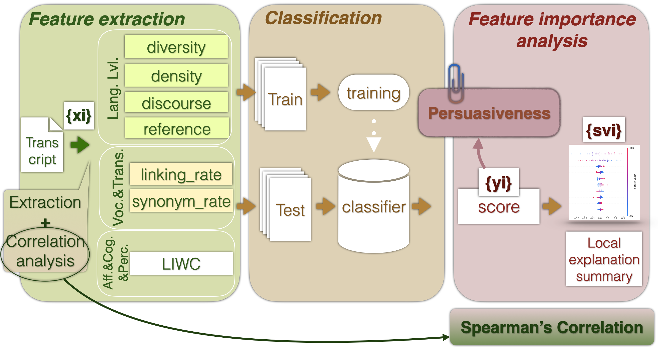
This repository contains code for extracting and evaluating the new public speaking textual feature set (PSTFS) on the performance classification task. PSTFS is tested on the 3MT_French dataset (collected from the competition "Ma thèse en 180 seconds") [@Biancardi2024]. The first results with PSTFS are reported in the paper [@Barkar2023] and published on ICMI2023. This repository contains updated results for further research.
The research paper [@Barkar2023] related to this project can be found here. A report with the updated detailed results can be found here
In [@Barkar2023] we consider two classes of performance quality: Data points with human-evaluated scores equal to or higher than the median were classified as "high-quality". In comparison, those with scores lower than the median were classified as "low-quality". In the update of this experiment, we study the following classification setups:
| Setup Keyword | Classes Sizes (Number of documents) |
|---|---|
| medianSep | (TODO:fill) |
| meanSep | (TODO:fill) |
| Q1Q3Sep | (TODO:fill) |
For class separation execute code preprocessing/LabelProcessor_MT.py with corresponding Setup Keyword. See the example for the separation w.r.t. median:
python3 LabelProcessor_MT.py --setup medianSep --dimension dimension_of_interest --clip fullHere, as dimension_of_interest put the name of the dimension that you are interested in (it will be persuasiveness by default):
| dimensions | options |
|---|---|
| persuasiveness | mean, rms, harmmean, rater1, rater2, rater3 |
| engagement | mean, rms, harmmean, rater1, rater2, rater3 |
| confidence | mean, rms, harmmean, rater1, rater2, rater3 |
| global | mean, rms, harmmean, rater1, rater2, rater3 |
mean: simple arithmetic mean rms: root mean squared harmmean: harmonic mean rater1: the rating of the first rater rater2: the rating of the second rater rate3: the rating of the third rater
You also can choose to work with the video clips (1 minute for the beginning, the middle and the end). The annotation schema for the clips was the same in the 3MT_French dataset, therefore, for each clip there are three raters to annotate it. All three raters always are different. For more details see [@Biancardi2024]. To switch to the clips you may use a clip with options: full, beg, mid, end. By default system will use "full".
Code with feature extraction is located in the file preprocessing/TextProcessor_MT.py. To execute it you can use the command:
python3 TextProcessor_MT.py --dataset MT "If you want to use the code on the other datasets then you should prepare input data so that:
- Transcripts are contained in the folder: '../data/{dataset}/transcripts/' where dataset is the name of the folder containing the transcripts of your dataset.
- Each transcript is located in the separated .txt file with the name corresponding to the ID of this sample in the dataset.
We used several classical classification models:
| Model | Parameters |
|---|---|
| Support Vector Machine (SVM) |
|
| Random Forest Classifier (RFC) |
|
| Logistic Regression (LR) |
|
| Naive Bayes (NB) | None |
| K-Nearest Neighbors (KNN) |
|
To test classification and obtain results one may use the following line executed from the root (default parameters: all, MT, persuasiveness, full):
python3 test_MT.py --model SVM --dataset MT --dimension dimension_of_interest --clip full| Parameter | Options |
|---|---|
| model | all, SVM, RFC, LR, NB, KNN |
| dataset | MT, POM |
| dimension |
|
| clip | full, beg, mid, end |
When the model is provided with the "all" option, the code will test all the classification models from this list: [SVM, RFC, LR, NB, KNN]. To add new models, please, add them to the file "./Models/ML_Model.py" and then to the list contained in the variable models_list in the test_MT.py.
SHAP value analysis is implemented in the same file with training and testing of the model, for more details refer to feedback/SHAP.py.
Finally, results will be saved to the folder: "results/{dataset}/classification/{rate_type} depending on which rate_type you specified above.
With any questions, you can contact me via alisa.barkar@talecom-paris.fr or alisa.george.barkar@gmail.com
