abdsamadf/grid-search-experiment

In this experiment we'll use Grid Search to find better parameters for this model, to reduce the overfitting.

Improving a model with Grid Search

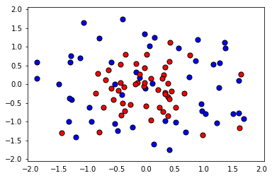
In this mini-lab, we'll fit a decision tree model to some sample data. This initial model will overfit heavily. Then we'll use Grid Search to find better parameters for this model, to reduce the overfitting.

First, some imports.

%matplotlib inline
import pandas as pd
import numpy as np
import matplotlib.pyplot as plt

1. Reading and plotting the data

Now, a function that will help us read the csv file, and plot the data.

def load_pts(csv_name):
    data = np.asarray(pd.read_csv(csv_name, header=None))
    X = data[:,0:2]
    y = data[:,2]

    plt.scatter(X[np.argwhere(y==0).flatten(),0], X[np.argwhere(y==0).flatten(),1],s = 50, color = 'blue', edgecolor = 'k')
    plt.scatter(X[np.argwhere(y==1).flatten(),0], X[np.argwhere(y==1).flatten(),1],s = 50, color = 'red', edgecolor = 'k')
    
    plt.xlim(-2.05,2.05)
    plt.ylim(-2.05,2.05)
    plt.grid(False)
    plt.tick_params(
        axis='x',
        which='both',
        bottom='off',
        top='off')

    return X,y

X, y = load_pts('data.csv')
plt.show()

2. Splitting our data into training and testing sets

from sklearn.model_selection import train_test_split
from sklearn.metrics import f1_score, make_scorer

#Fixing a random seed
import random
random.seed(42)

# Split the data into training and testing sets
X_train, X_test, y_train, y_test = train_test_split(X, y, test_size=0.2, random_state=42)

3. Fitting a Decision Tree model

from sklearn.tree import DecisionTreeClassifier

# Define the model (with default hyperparameters)
clf = DecisionTreeClassifier(random_state=42)

# Fit the model
clf.fit(X_train, y_train)

# Make predictions
train_predictions = clf.predict(X_train)
test_predictions = clf.predict(X_test)

Now let's plot the model, and find the testing f1_score, to see how we did.

The following function will help us plot the model.

def plot_model(X, y, clf):
    plt.scatter(X[np.argwhere(y==0).flatten(),0],X[np.argwhere(y==0).flatten(),1],s = 50, color = 'blue', edgecolor = 'k')
    plt.scatter(X[np.argwhere(y==1).flatten(),0],X[np.argwhere(y==1).flatten(),1],s = 50, color = 'red', edgecolor = 'k')

    plt.xlim(-2.05,2.05)
    plt.ylim(-2.05,2.05)
    plt.grid(False)
    plt.tick_params(
        axis='x',
        which='both',
        bottom='off',
        top='off')

    r = np.linspace(-2.1,2.1,300)
    s,t = np.meshgrid(r,r)
    s = np.reshape(s,(np.size(s),1))
    t = np.reshape(t,(np.size(t),1))
    h = np.concatenate((s,t),1)

    z = clf.predict(h)

    s = s.reshape((np.size(r),np.size(r)))
    t = t.reshape((np.size(r),np.size(r)))
    z = z.reshape((np.size(r),np.size(r)))

    plt.contourf(s,t,z,colors = ['blue','red'],alpha = 0.2,levels = range(-1,2))
    if len(np.unique(z)) > 1:
        plt.contour(s,t,z,colors = 'k', linewidths = 2)
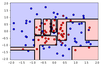
    plt.show()

plot_model(X, y, clf)
print('The Training F1 Score is', f1_score(train_predictions, y_train))
print('The Testing F1 Score is', f1_score(test_predictions, y_test))

The Training F1 Score is 1.0
The Testing F1 Score is 0.7

Woah! Some heavy overfitting there. Not just from looking at the graph, but also from looking at the difference between the high training score (1.0) and the low testing score (0.7).Let's see if we can find better hyperparameters for this model to do better. We'll use grid search for this.

4. (TODO) Use grid search to improve this model.

In here, we'll do the following steps:

1. First define some parameters to perform grid search on. We suggest to play with max_depth, min_samples_leaf, and min_samples_split.
2. Make a scorer for the model using f1_score.
3. Perform grid search on the classifier, using the parameters and the scorer.
4. Fit the data to the new classifier.
5. Plot the model and find the f1_score.
6. If the model is not much better, try changing the ranges for the parameters and fit it again.

Hint: If you're stuck and would like to see a working solution, check the solutions notebook in this same folder.

from sklearn.metrics import make_scorer
from sklearn.model_selection import GridSearchCV

clf = DecisionTreeClassifier(random_state=42)

# TODO: Create the parameters list you wish to tune.
parameters = {'max_depth':[1,2,3,4,5], 'min_samples_leaf':[1,2,3,4,5], 'min_samples_split':[2,3,4,5] }

# TODO: Make an fbeta_score scoring object.
from sklearn.metrics import make_scorer 
from sklearn.metrics import f1_score 
scorer = make_scorer(f1_score)

# TODO: Perform grid search on the classifier using 'scorer' as the scoring method.
grid_obj = GridSearchCV(clf, parameters, scoring=scorer)

# TODO: Fit the grid search object to the training data and find the optimal parameters.
grid_fit = grid_obj.fit(X, y)

# TODO: Get the estimator.
best_clf = grid_fit.best_estimator_

# Fit the new model.
best_clf.fit(X_train, y_train)

# Make predictions using the new model.
best_train_predictions = best_clf.predict(X_train)
best_test_predictions = best_clf.predict(X_test)

# Calculate the f1_score of the new model.
print('The training F1 Score is', f1_score(best_train_predictions, y_train))
print('The testing F1 Score is', f1_score(best_test_predictions, y_test))

# Plot the new model.
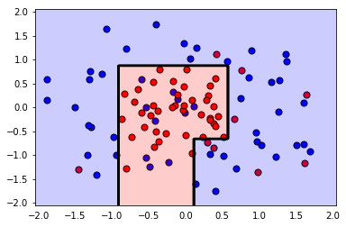
plot_model(X, y, best_clf)

# Let's also explore what parameters ended up being used in the new model.
best_clf

The training F1 Score is 0.814814814815
The testing F1 Score is 0.8

DecisionTreeClassifier(class_weight=None, criterion='gini', max_depth=4,
            max_features=None, max_leaf_nodes=None,
            min_impurity_decrease=0.0, min_impurity_split=None,
            min_samples_leaf=4, min_samples_split=2,
            min_weight_fraction_leaf=0.0, presort=False, random_state=42,
            splitter='best')

Conclusion:

Note that by using GridSearch we improved the F1 Score from 0.7 to 0.8 (and we lost some training score, but this is ok). Also, if you look at the plot, the second model has a much simpler boundary, which implies that it's less likely to overfit.